3. General Features

This section explains features common to all the programs in GMT and summarizes the philosophy behind the system. Some of the features described here may make more sense once you reach the cook-book section where we present actual examples of their use.

3.1. GMT Modern Mode Hierarchical Levels

As you read below of how we handle default settings, command-line history, and color tables, it is important to understand that under GMT modern mode we maintain several levels of these parameters. As you will see later, this affects three aspects of GMT: The chosen default settings, the current history of previous common option arguments, and the current color table. All three items are given a consistent treatment in GMT modern mode (in classic mode there is only a single level and no concept of a current color table). Below, item refers to any of those three aspects.

1. The top level is the session. Any item set here is accessible to all other levels.

2. The next level is the figure level. A session may create numerous figures and items determined at this level are only accessible to that figure and plot constructs below it (like subplots).

3. A figure may include a subplot. Before any panels are started, any items determined at this level apply to all the panels in the subplot. For instance, setting a new color table will apply to all the panels that need it.

4. Once you start a specific panel in a subplot, any items determined at this level only apply to that panel. For instance, changing the font used for frame annotations for this panel is not affecting any other panels.

5. Figures or panels may include a map inset. Any items determined in an inset is private to that inset and does not affect the higher levels.

There is a distinction between setting an item (e.g., a font choice, an option like plot region, or a color table) and getting that item. When we specify a particular item it is recorded at that level. When we need to access that item, there may or may not be an item at the current hierarchical level. If there is not, we look at the level above the current level to see if it has the required item, and this search may go all the way back to the session level. In other words, we always give preference to items set at or just above the current hierarchical level as possible. If no such item is found anywhere then we use the GMT defaults or color table, or we must terminate with an error if a required setting such as a region cannot be determined from your options or data sets.

Discussions below on GMT defaults and history are presented as they apply to classic mode, but under modern mode these files are maintained at the levels we just discussed.

3.2. GMT units

While GMT has default units for both actual Earth distances and plot lengths (i.e., dimensions) of maps, it is recommended that you explicitly indicate the units of your arguments by appending the unit character, as discussed below. This will aid you in debugging, let others understand your scripts, and remove any uncertainty as to what unit you thought you wanted.

3.2.1. Dimension units

GMT programs accept plot dimensional quantities (widths, offsets, etc.) in cm, inch, or point (1/72 of an inch) [8]. There are two ways to ensure that GMT understands which unit you intend to use:

1. Append the desired unit to the dimension you supply. This way is explicit and clearly communicates what you intend, e.g., -JM10c means the map width being passed to the -JM switch is 10 cm, and modifier +o24p means we are offsetting a feature by 24 points from its initial location.

2. Set the parameter PROJ_LENGTH_UNIT to the desired unit. Then, all dimensions without explicit units will be interpreted accordingly. By default, GMT always initializes PROJ_LENGTH_UNIT to cm and interprets unitless dimensional values as cm, except for fonts and pen thicknesses which are by default interpreted as points.

The latter method is less robust as other users may have a different default unit set and then your script may not work as intended. For portability, we therefore recommend you always append the desired unit explicitly.

3.2.2. Distance units

d	Degree of arc	M	Statute mile
e	Meter [Default]	n	Nautical mile
f	Foot	s	Second of arc
k	Kilometer	u	US Survey foot
m	Minute of arc

For Cartesian data the data units do not normally matter (they could be kg or Lumens for all we know) and are never entered. Geographic data are different, as distances can be specified in a variety of ways. GMT programs that accept actual Earth length scales like search radii or distances can therefore handle a variety of units. These choices are listed in the Table Distance Units; simply append the desired unit to the distance value you supply. A value without a unit suffix will be consider to be in meters. For example, a distance of 30 nautical miles should be given as 30n.

3.2.3. Distance calculations

The calculation of distances on Earth (or other planetary bodies) depends on the ellipsoidal parameters of the body (via PROJ_ELLIPSOID) and the method of computation. GMT offers three alternatives that trade off accuracy and computation time.

3.2.3.1. Flat Earth distances

Quick, but approximate “Flat Earth” calculations make a first-order correction for the spherical nature of a planetary body by computing the distance between two points A and B as

\[d_f = R \sqrt{(\theta_A - \theta_B)^2 + (\cos \left [ \frac{\theta_A + \theta_B}{2} \right ] \Delta \lambda)^2}, \label{eq:flatearth}\]

where R is the representative (or spherical) radius of the planet, \(\theta\) is latitude, and the difference in longitudes, \(\Delta \lambda = \lambda_A - \lambda_B\), is adjusted for any jumps that might occur across Greenwich or the Dateline. As written, the geographic coordinates are given in radians. This approach is suitable when the points you use to compute \(d_f\) do not greatly differ in latitude and computation speed is paramount. You can select this mode of computation by specifying the common GMT option -j and appending the directive f (for Flat Earth). For instance, a search radius of 50 statute miles using this mode of computation might be specified via -S50M -jf.

3.2.3.2. Great circle distances

This is the default distance calculation, which will also approximate the planetary body by a sphere of mean radius R. However, we compute an exact distance between two points A and B on such a sphere via the Haversine equation

\[d_g = 2R \sin^{-1} {\sqrt{\sin^2\frac{\theta_A - \theta_B}{2} + \cos \theta_A \cos \theta_B \sin^2 \frac{\lambda_A - \lambda_B}{2}} }, \label{eq:greatcircle}\]

This approach is suitable for most situations unless exact calculations for an ellipsoid is required (typically for a limited surface area). For instance, a search radius of 5000 feet using this mode of computation would be specified as -S5000f.

Note: There are two additional GMT defaults that control how great circle (and Flat Earth) distances are computed. One concerns the selection of the “mean radius”. This is selected by PROJ_MEAN_RADIUS, which selects one of several possible representative radii. The second is PROJ_AUX_LATITUDE, which converts geodetic latitudes into one of several possible auxiliary latitudes that are better suited for the spherical approximation. While both settings have default values to best approximate geodesic distances (authalic mean radius and latitudes), expert users can choose from a range of options as detailed in the gmt.conf man page. Note that these last two settings are only used if the PROJ_ELLIPSOID is not set to “sphere”.

3.2.3.3. Geodesic distances

For the most accurate calculations we use a full ellipsoidal formulation. Currently, we are using Vincenty’s [1975] formula [7] which is accurate to 0.5 mm. You select this mode of computation by using the common GMT option -j and appending the directive e (for ellipsoidal). For instance, a search radius of 20 km using this mode of computation would be set by -S20k -je. You may use the setting PROJ_GEODESIC which defaults to Vincenty but may also be set to Rudoe for old GMT4-style calculations or Andoyer for an approximate geodesic (within a few tens of meters) that is much faster to compute.

3.3. GMT defaults

3.3.1. Overview and the gmt.conf file

There are almost 150 parameters which can be adjusted individually to modify the appearance of plots or affect the manipulation of data. When a new session starts (unless -C is given), it initializes all parameters to the GMT defaults [9], then tries to open the file gmt.conf in the current directory [10]. If not found, it will look for that file in a sub-directory .gmt of your home directory, and finally in your home directory itself. If successful, the session will read the contents and set the default values to those provided in the file. By editing this file you can affect features such as pen thicknesses used for maps, fonts and font sizes used for annotations and labels, color of the pens, dots-per-inch resolution of the hardcopy device, what type of spline interpolant to use, and many other choices. A complete list of all the parameters and their default values can be found in the gmt.conf manual pages. Figures GMT Parameters a, b, and c show the parameters that affect plots. You may create your own gmt.conf files by running gmtdefaults and then modify those parameters you want to change. If you want to use the parameter settings in another file you can do so by copying that file to the current directory and call it gmt.conf. This makes it easy to maintain several distinct parameter settings, corresponding perhaps to the unique styles required by different journals or simply reflecting font changes necessary to make readable overheads and slides. At the end of such scripts you should then delete the (temporary) gmt.conf file. Note that any arguments given on the command line (see below) will take precedent over the default values. E.g., if your gmt.conf file has x offset = 3c as default, the -X5c option will override the default and set the offset to 5 cm.

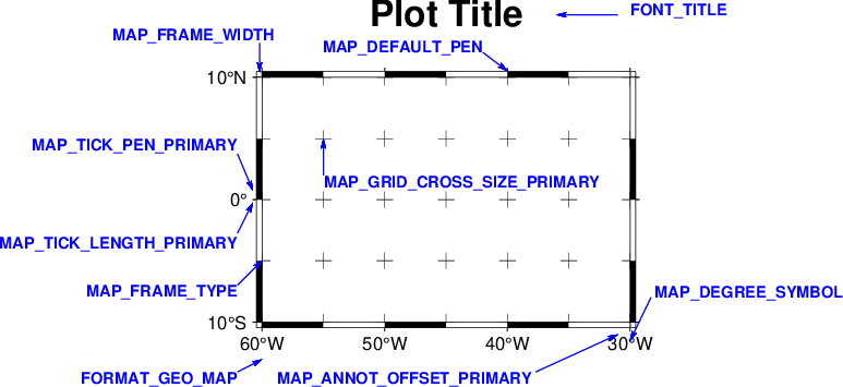
Some GMT parameters that affect plot appearance.

Here is the source script for the figure above:

gmt begin GMT_Defaults_1a
	gmt set GMT_THEME cookbook
	gmt set MAP_FRAME_TYPE fancy FORMAT_GEO_MAP ddd:mm:ssF MAP_GRID_CROSS_SIZE_PRIMARY 0.1i FONT_ANNOT_PRIMARY +8p
	gmt basemap -X2i -R-60/-30/-10/10 -JM2.25i -Ba10f5g5 -BWSne+t"Plot Title"
	gmt text -N -F+f7p,Helvetica-Bold,blue+j << EOF
-62  -7 RT MAP_FRAME_TYPE
-38 -14 RT MAP_ANNOT_OFFSET_PRIMARY
-62  -3 RT MAP_TICK_LENGTH_PRIMARY
-62   4 RB MAP_TICK_PEN_PRIMARY
-59  13 RB MAP_FRAME_WIDTH
-42  12 RB MAP_DEFAULT_PEN
-55   2 LT MAP_GRID_CROSS_SIZE_PRIMARY
-30  15 LB FONT_TITLE
-62 -14 RT FORMAT_GEO_MAP
-28  -8 LB MAP_DEGREE_SYMBOL
EOF
	gmt plot -Sv0.06i+s+e -W0.5p,blue -N -Gblue << EOF
-62 -7 -60 -5
-37.7 -14 -31 -11
-62 -2.75 -60.75 -0.25
-62 3.75 -60.75 0.75
-42 12 -40 10.5
-55 2 -55 5
-31 15 -36 15
-60.20 12.75 -60.20 10.4
-62 -14 -60 -13
-28.3 -8 -30 -11.5
EOF
gmt end show

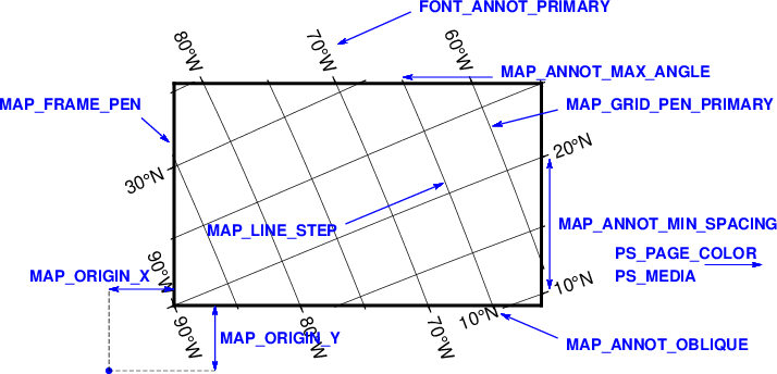
More GMT parameters that affect plot appearance.

Here is the source script for the figure above:

gmt begin GMT_Defaults_1b
	gmt set GMT_THEME cookbook
	gmt set MAP_FRAME_TYPE plain FORMAT_GEO_MAP ddd:mm:ssF MAP_GRID_CROSS_SIZE_PRIMARY 0i \
		FONT_ANNOT_PRIMARY +8p MAP_ANNOT_OBLIQUE anywhere MAP_FRAME_AXES=WESN
	gmt basemap -X1.5i -R-90/20/-55/25+r -JOc-80/25.5/2/69/2.25i -Ba10f5g5
	gmt text -R0/2.25/0/2 -Jx1i -N -F+f7p,Helvetica-Bold,blue+j << EOF
-0.15 0.15  RB MAP_ORIGIN_X
0.28  -0.2  LM MAP_ORIGIN_Y
-0.2   1.2  RB MAP_FRAME_PEN
2.4   -0.2  LT MAP_ANNOT_OBLIQUE
2.4    1.2  LB MAP_GRID_PEN_PRIMARY
2      1.4  LB MAP_ANNOT_MAX_ANGLE
2.35   0.5  LM MAP_ANNOT_MIN_SPACING
1      0.5  RT MAP_LINE_STEP
2.7    0.32 LM PS_PAGE_COLOR
2.7    0.18 LM PS_MEDIA
1.5     1.8 LB FONT_ANNOT_PRIMARY
EOF
	echo -0.4 -0.4 | gmt plot -Sc0.04i -Gblue -N
	gmt plot -Sv0.06i+s+b+e -N -W0.5p,blue -Gblue << EOF
0 0.1 -0.4 0.1
0.25 0 0.25 -0.4
2.3 0.1 2.3 0.9
EOF
	gmt plot -Sv0.06i+s+e -N -W0.5p,blue -Gblue << EOF
-0.2 1.15 -0.03 1
2.35 -0.2 2.0 -0.05
2.35 1.2 1.95 1.1
1.95 1.4 1.4 1.4
1.05 0.5 1.65 0.75
3.25 0.25 3.6 0.25
1.45 1.8 1 1.6
EOF
	gmt plot -Wthinnest,- -X-0.5i -Y-0.5i << EOF
>
0.1	0.1
0.1	0.6
>
0.1	0.1
0.75	0.1
EOF
gmt end show

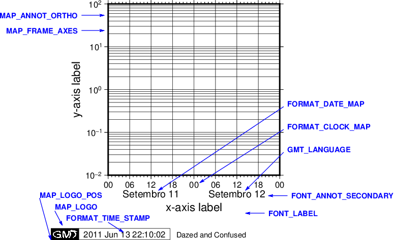
Even more GMT parameters that affect plot appearance.

Here is the source script for the figure above:

gmt begin GMT_Defaults_1c
	gmt set GMT_THEME cookbook
	gmt set MAP_FRAME_TYPE plain FORMAT_DATE_MAP "o dd" FORMAT_CLOCK_MAP hh FONT_ANNOT_PRIMARY +8p
	gmt basemap -R2001-9-11T/2001-9-13T/0.01/100 -JX2.25iT/2.25il -Bpxa6Hf1hg6h+l"x-axis label" -Bpya1g3p+l"y-axis label" -BWSne \
		-X2i -Bsxa1D -U"Dazed and Confused"+o-0.75i/-0.85i --GMT_LANGUAGE=pt \
		--FORMAT_TIME_STAMP="2011 Jun 13 22:10:02"
	gmt text -R0/2.25/0/2.25 -Jx1i -N -F+f7p,Helvetica-Bold,blue+j << EOF
-0.4   2.1 RM MAP_ANNOT_ORTHO
-0.4   1.9 RM MAP_FRAME_AXES
-0.9  -0.3 LB MAP_LOGO_POS
-0.7 -0.45 LB MAP_LOGO
0.0   -0.6 CB FORMAT_TIME_STAMP
2.1   -0.5 LM FONT_LABEL
2.35   0.9 LB FORMAT_DATE_MAP
2.35   0.6 LB FORMAT_CLOCK_MAP
2.35   0.3 LB GMT_LANGUAGE
2.4   -0.27 LM FONT_ANNOT_SECONDARY
EOF
	gmt plot -Sv0.06i+s+e -N -W0.5p,blue -Gblue << EOF
-0.35 2.1 -0.05 2.1
-0.35 1.9 -0.05 1.9
-0.9 -0.3 -0.75 -0.85
-0.7 -0.47 -0.6 -0.66
0.0 -0.62 0.2 -0.75
2.05 -0.5 1.8 -0.5
2.3 0.9 0.66 -0.2
2.3 0.6 1.2 -0.1
2.3 0.3 1.8 -0.2
2.35 -0.27 2.1 -0.27
EOF
gmt end show

There are at least two good reasons why the GMT default options are placed in a separate parameter file:

1. It would not be practical to allow for command-line syntax covering so many options, many of which are rarely or never changed (such as the ellipsoid used for map projections).

2. It is convenient to keep separate gmt.conf files for specific projects, so that one may achieve a special effect simply by running GMT commands in the directory whose gmt.conf file has the desired settings. For example, when making final illustrations for a journal article one must often standardize on font sizes and font types, etc. Keeping all those settings in a separate gmt.conf file simplifies this process and will allow you to generate those illustrations with the same settings later on. Likewise, GMT scripts that make figures for PowerPoint presentations often use a different color scheme and font size than output intended for laser printers. Organizing these various scenarios into separate gmt.conf files will minimize headaches associated with micro-editing of illustrations.

3.3.2. Automatic GMT settings

The auto flag for GMT parameters signals that suitable dimensions or settings will be automatically computed when the plot dimensions are known. The auto flag is supported for the following parameters:

FONT_ANNOT_PRIMARY	Primary annotation font [11.00p]
FONT_ANNOT_SECONDARY	Secondary annotation font [13.20p]
FONT_HEADING	Subplot heading font [30.80p]
FONT_LABEL	Axis label font [15.40p]
FONT_LOGO	Logo font [8.80p]
FONT_SUBTITLE	Plot subtitle font [19.80p]
FONT_TAG	Tag/labeling font [17.60p]
FONT_TITLE	Plot title font [24.20p]
MAP_ANNOT_MIN_SPACING	Minimum space between annotations [11.00p]
MAP_ANNOT_OFFSET_PRIMARY	Primary annotation offset from axis [3.30p]
MAP_ANNOT_OFFSET_SECONDARY	Secondary annotation offset from axis [3.30p]
MAP_EMBELLISHMENT_MODE	Scales attributes relative to feature size
MAP_FRAME_AXES	Axes that are drawn and annotated
MAP_FRAME_PEN	Pen width of plain frame [1.65p]
MAP_FRAME_WIDTH	Width of fancy frame [3.30p]
MAP_GRID_PEN_PRIMARY	Pen width of primary gridline [0.28p]
MAP_GRID_PEN_SECONDARY	Pen width of secondary gridline [0.55p]
MAP_HEADING_OFFSET	Heading offset from subplot [17.60p]
MAP_LABEL_OFFSET	Label offset from annotations [6.60p]
MAP_POLAR_CAP	Appearance of gridlines near the poles
MAP_TICK_LENGTH_PRIMARY	Length of primary tick marks [2.2p/1.1p]
MAP_TICK_LENGTH_SECONDARY	Length of secondary tick marks [6.60p/1.65p]
MAP_TICK_PEN_PRIMARY	Pen width of primary tick marks [0.55p]
MAP_TICK_PEN_SECONDARY	Pen width of secondary tick marks [0.28p]
MAP_TITLE_OFFSET	Title offset from plot [13.20p]

The reference dimensions listed in brackets are the values for a plot with a height and width of 25 cm. Larger and smaller illustrations will see a linear magnification or attenuation of these dimensions. The primary annotation font size will be computed as:

size = (2/15) * (map_size_in_cm - 10) + 9 [in points]

where \(map\_size\_in\_cm = \sqrt(map\_height \times map\_width)\). All other items will have their reference sizes scaled by \(scale = size / 10\). In modern mode, if you do nothing then all of the above dimensions will be automatically set based on your plot dimensions. However, you are free to override any of them using the methods described in the next section. Note: Selecting auto for font sizes and dimensions requires GMT to know the plot dimensions. If the plot dimensions are not available (e.g., pslegend with -Dx and no -R -J), the settings will be updated using the nominal font sizes and dimensions for a 10 x 1 cm plot. Note: The particular scaling relationship is experimental in 6.2 and we reserve the right to adjust it pending further experimentation and user feedback.

For MAP_POLAR_CAP, auto will determine a suitable pc_lat for your region for all azimuthal projections and a few others in which the geographic poles are plotted as points (Lambert Conic, Oblique Mercator, Hammer, Mollweide, Sinusoidal, and van der Grinten).

For MAP_FRAME_AXES, auto will determine a suitable setting based on the projection, type of plot, perspective, etc. For example, GMT will determine the position of different quadrants for perspective and polar plots and select the equivalent of WrStZ. The default for the Gnomonic and general perspective projections is WESNZ. The default for non-perspective, non-Gnomonic, and non-polar plots using MAP_FRAME_AXES=auto is WrStZ.

For MAP_LABEL_OFFSET, auto will scale the offset based on figure size if MAP_LABEL_MODE is set to annot, but will default to 32p if :term:MAP_LABEL_MODE` is set to axis.

For MAP_EMBELLISHMENT_MODE, auto means we uses the given size of the embellishment to set relative sizes of ticks, texts and labels, and offsets. These are otherwise controlled by numerous default settings; see discussion under Embellishments.

3.3.3. Changing GMT defaults

As mentioned, GMT programs will attempt to open a file named gmt.conf. At times it may be desirable to override that default. There are several ways in which this can be accomplished.

• One method is to start each script by saving a copy of the current gmt.conf, then copying the desired gmt.conf file to the current directory, and finally reverting the changes at the end of the script. Possible side effects include premature ending of the script due to user error or bugs which means the final resetting does not take place (unless you write your script very carefully.)

• To permanently change some of the GMT parameters on the fly inside a script the gmtset utility can be used. E.g., to change the primary annotation font to 12 point Times-Bold in red we run

  gmt set FONT_ANNOT_PRIMARY 12p,Times-Bold,red
  

  These changes will remain in effect until they are overridden.

• If all you want to achieve is to change a few parameters during the execution of a single command but otherwise leave the environment intact, consider passing the parameter changes on the command line via the --PAR=value mechanism. For instance, to temporarily set the output format for floating points to have lots of decimals, say, for map projection coordinate output, append --FORMAT_FLOAT_OUT=%.16lg to the command in question.

In addition to those parameters that directly affect the plot there are numerous parameters than modify units, scales, etc. For a complete listing, see the gmt.conf man pages. We suggest that you go through all the available parameters at least once so that you know what is available to change via one of the described mechanisms. The gmt.conf file can be cleared by running gmt clear settings.

3.4. Command line arguments

Each program requires certain arguments specific to its operation. These are explained in the manual pages and in the usage messages. We have tried to choose letters of the alphabet which stand for the argument so that they will be easy to remember. Each argument specification begins with a hyphen (except input file names; see below), followed by a letter, and sometimes a number or character string immediately after the letter. Do not space between the hyphen, letter, and number or string. Do space between options. Example:

gmt coast -R0/20/0/20 -Ggray -JM15c -Wthin -Baf -V -pdf map

3.5. Command line history

GMT programs “remember” the standardized command line options (See Chapter Standardized command line options) given during their first invocations in a modern mode session, and afterwards we do not need to repeat them any further. For example, if a map was created with an Cartesian linear projection, then any subsequent plot commands to plot symbols on the same map do not need to repeat the region and projection information, as shown here:

gmt begin map
  gmt basemap -R0/6.5/0/7 -Jx2c -B
  gmt plot @Table_5_11.txt -Sc0.3c -Gred
gmt end show

Thus, the chosen options remain in effect until you provide new option arguments on the command line. Note: We keep track of two types of regions, One is the domain used for a map and one is the domain used for processing, which often are the same. When a plot is specified without providing a region then we look for a previous plot region in the history first, and if it is not found then we look for the processing domain to use instead. However, if a data-processing module is not given a region then we only look for a previous processing domain; we never substitute a plot domain in that case.

3.6. Usage messages, syntax- and general error messages

Each program carries a usage message. If you enter the program name without any arguments, the program will write the complete usage message to standard error (your screen, unless you redirect it). This message explains in detail what all the valid arguments are. If you enter the program name followed by a hyphen (-) only you will get a shorter version which only shows the command line syntax and no detailed explanations. If you incorrectly specify an option or omit a required option, the program will produce syntax errors and explain what the correct syntax for these options should be. If an error occurs during the running of a program, the program will in some cases recognize this and give you an error message. Usually this will also terminate the run. The error messages generally begin with the name of the program in which the error occurred; if you have several programs piped together this tells you where the trouble is.

3.7. Standard input or file, header records

Most of the programs which expect table data input can read either standard input or input in one or several files. These programs will try to read standard input unless you type the filename(s) on the command line without the above hyphens. (If the program sees a hyphen, it reads the next character as an instruction; if an argument begins without a hyphen, it tries to open this argument as a filename). This feature allows you to connect programs with pipes if you like. To give numerous input files you can either list them all (file1.txt file2.txt …), use UNIX wild cards (file*.txt), or make a simple listfile with the names of all your datafiles (one per line) and then use the special =filelist mechanism to specify the input files to a module. This allows GMT modules to obtain the input file names from filelist. If your input is ASCII and has one or more header records that do not begin with #, you must use the -h option (see Section Header data records: The -h option). ASCII files may in many cases also contain segment-headers separating data segments. These are called “multi-segment files”. For binary table data the -h option may specify how many bytes should be skipped before the data section is reached. Binary files may also contain segment-headers separating data segments. These segment-headers are simply data records whose fields are all set to NaN; see Chapter GMT File Formats for complete documentation.

If filenames are given for reading, GMT programs will first look for them in the current directory. If the file is not found, the programs will look in other directories pointed to by the directory parameters DIR_DATA and DIR_CACHE or by the environmental parameters $GMT_USERDIR, $GMT_CACHEDIR and $GMT_DATADIR (if set). They may be set by the user to point to directories that contain data sets of general use, thus eliminating the need to specify a full path to these files. Usually, the DIR_DATA directory will hold data sets of a general nature (tables, grids), whereas the $GMT_USERDIR directory (its default value is $HOME/.gmt) may hold miscellaneous data sets more specific to the user; this directory also stores GMT defaults, other configuration files and modern session directories as well as the directory server which olds downloaded data sets from the GMT data server The DIR_CACHE will typically contain other data files downloaded when running tutorial or example scripts. See directory parameters for details. Program output is always written to the current directory unless a full path has been specified.

3.8. URLs and remote files

Three classes of files are given special treatment in GMT.

1. Some data sets are ubiquitous and used by nearly all GMT users. At the moment this collection is limited to Earth relief grids. If you specify a grid input named @earth_relief_res on a command line then such a grid will automatically be downloaded from the GMT Data Server and placed in the server directory under $GMT_USERDIR [~/.gmt]. The resolution res allows a choice among 15 common grid spacings: 01d, 30m, 20m, 15m, 10m, 06m, 05m, 04m, 03m, 02m, 01m, 30s, and 15s (with file sizes 111 kb, 376 kb, 782 kb, 1.3 Mb, 2.8 Mb, 7.5 Mb, 11 Mb, 16 Mb, 27 Mb, 58 Mb, 214 Mb, 778 Mb, and 2.6 Gb respectively) as well as the SRTM tile resolutions 03s and 01s (6.8 Gb and 41 Gb for the whole set, respectively). Once one of these grids have been downloaded any future reference will simply obtain the file from $GMT_USERDIR (except if explicitly removed by the user). Note: The 15 arc-sec data comes from the original dataset SRTM15+. Lower resolutions are spherically Gaussian-filtered versions of SRTM15+. The SRTM (version 3) 1 and 3 arc-sec tiles are only available over land between 60 degrees south and north latitude and are stored as highly compressed JPEG2000 tiles on the GMT server. These are individually downloaded as requested, converted to netCDF grids and stored in subdirectories srtm1 and srtm3 under the server directory, and assembled into a seamless grid using grdblend. A tile is only downloaded and converted once (unless the user cleans the data directories).

2. If a file is given as a full URL, starting with http://, https://, or ftp://, then the file will be downloaded to the current directory and subsequently read from there (until removed by the user). If the URL is actually a CGI Get command (i.e., ends in ?par=val1&par2=val2…) then we download the file each time we encounter the URL.

3. Demonstration files used in online documentation, example scripts, or even the large test suite may be given in the format @filename. When such a file is encountered on the command line it is understood to be a short-hand representation of the full URL to filename on the GMT Cache Data site. Since this address may change over time we use the leading @ to simplify access to these files. Such files will also be downloaded to DIR_CACHE and subsequently read from there (until removed by the user).

4. By default, remote files are downloaded from the SOEST data server. However, you can override that selection by setting the environmental parameter $GMT_DATA_SERVER or the default setting for GMT_DATA_SERVER. Alternatively, configure the CMake parameter GMT_DATA_SERVER at compile time.

5. If your Internet connection is slow or nonexistent (e.g., on a plane) you can also limit the size of the largest datafile to download via GMT_DATA_SERVER_LIMIT or you can temporarily turn off such downloads by setting GMT_DATA_UPDATE_INTERVAL to “off”.

The user cache (DIR_CACHE) and all its contents can be cleared any time via the command gmt clear cache, while the server directory with downloaded data can be cleared via the command gmt clear data. Finally, when a remote file is requested we also check if that file has changed at the server and re-download the updated file; this check is only performed no more often than once a day.

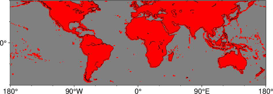
The 14297 1x1 degree tiles (red) for which SRTM 1 and 3 arc second data are available.

Here is the source script for the figure above:

gmt begin GMT_SRTM
	gmt set GMT_THEME cookbook
	gmt set MAP_FRAME_TYPE plain
	gmt coast -R-180/180/-60/60 -JQ0/15c -B -BWStr -Dc -A5000 -Glightgray --FORMAT_GEO_MAP=dddF
	echo "1	red 2 red" > t.cpt
	gmt grdmath @srtm_tiles.nc 0 NAN = t.nc
	gmt grdimage t.nc -Ct.cpt
	gmt coast -Dc -A5000 -W0.25p
gmt end show

As a short example, we can make a quick map of Easter Island using the SRTM 1x1 arc second grid via

gmt grdimage -R109:30W/109:12W/27:14S/27:02S -JM15c -B @earth_relief_01s -png easter

3.9. Verbose operation

Most of the programs take an optional -V argument which will run the program in the “verbose” mode (see Section Verbose feedback: The -V option). Verbose will write to standard error information about the progress of the operation you are running. Verbose reports things such as counts of points read, names of data files processed, convergence of iterative solutions, and the like. Since these messages are written to stderr, the verbose talk remains separate from your data output. You may optionally choose among six models of verbosity; each mode adds more messages with an increasing level of details. The modes are

• q - Quiet, not even fatal error messages are produced.

• e - Error messages only.

• w - Warnings (same as running without -V)

• t - Timings (report runtimes for time-intensive algorithms).

• i - Informational messages (same as -V only).

• c - Compatibility warnings (if compiled with backward-compatibility).

• d - Debugging messages (mostly of interest to developers).

The verbosity is cumulative, i.e., mode w means all messages of mode e as well will be reported.

3.10. Program output

Most programs write their results, including PostScript plots, to standard output. The exceptions are those which may create binary netCDF grid files such as surface (due to the design of netCDF a filename must be provided; however, alternative binary output formats allowing piping are available; see Section Grid file format specifications). Most operating systems let you can redirect standard output to a file or pipe it into another process. Error messages, usage messages, and verbose comments are written to standard error in all cases. You can usually redirect standard error as well, if you want to create a log file of what you are doing. The syntax for redirection differ among the main shells (Bash and C-shell) and is a bit limited in DOS.

3.11. Input data formats

Most of the time, GMT will know what kind of x and y coordinates it is reading because you have selected a particular coordinate transformation or map projection. However, there may be times when you must explicitly specify what you are providing as input using the -f switch. When binary input data are expected (-bi) you must specify exactly the format of the records. However, for ASCII input there are numerous ways to encode data coordinates (which may be separated by white-space or commas). Valid input data are generally of the same form as the arguments to the -R option (see Section Data domain or map region: The -R option), with additional flexibility for calendar data. Geographical coordinates, for example, can be given in decimal degrees (e.g., -123.45417) or in the [±]ddd[:mm[:ss[.xxx]]][W|E|S|N] format (e.g., 123:27:15W). With -fp you may even supply projected data like UTM coordinates.

Because of the widespread use of incompatible and ambiguous formats, the processing of input date components is guided by the template FORMAT_DATE_IN in your gmt.conf file; it is by default set to yyyy-mm-dd. Y2K-challenged input data such as 29/05/89 can be processed by setting FORMAT_DATE_IN to dd/mm/yy. A complete description of possible formats is given in the gmt.conf man page. The clock string is more standardized but issues like 12- or 24-hour clocks complicate matters as well as the presence or absence of delimiters between fields. Thus, the processing of input clock coordinates is guided by the template FORMAT_CLOCK_IN which defaults to hh:mm:ss.xxx.

GMT programs that require a map projection argument will implicitly know what kind of data to expect, and the input processing is done accordingly. However, some programs that simply report on minimum and maximum values or just do a reformatting of the data will in general not know what to expect, and furthermore there is no way for the programs to know what kind of data other columns (beyond the leading x and y columns) contain. In such instances we must explicitly tell GMT that we are feeding it data in the specific geographic or calendar formats (floating point data are assumed by default). We specify the data type via the -f option (which sets both input and output formats; use -fi and -fo to set input and output separately). For instance, to specify that the the first two columns are longitude and latitude, and that the third column (e.g., z) is absolute calendar time, we add -fi0x,1y,2T to the command line. For more details, see the man page for the program you need to use.

3.12. Output data formats

The numerical output from GMT programs can be binary (when -bo is used) or ASCII [Default]. In the latter case the issue of formatting becomes important. GMT provides extensive machinery for allowing just about any imaginable format to be used on output. Analogous to the processing of input data, several templates guide the formatting process. These are FORMAT_DATE_OUT and FORMAT_CLOCK_OUT for calendar-time coordinates, FORMAT_GEO_OUT for geographical coordinates, and FORMAT_FLOAT_OUT for generic floating point data. In addition, the user have control over how columns are separated via the IO_COL_SEPARATOR parameter. Thus, as an example, it is possible to create limited FORTRAN-style card records by setting FORMAT_FLOAT_OUT to %7.3lf and IO_COL_SEPARATOR to none [Default is tab].

3.13. PostScript features

PostScript is a command language for driving graphics devices such as laser printers. It is ASCII text which you can read and edit as you wish (assuming you have some knowledge of the syntax). We prefer this to binary metafile plot systems since such files cannot easily be modified after they have been created. GMT programs also write many comments to the plot file which make it easier for users to orient themselves should they need to edit the file (e.g., % Start of x-axis) [16]. All GMT programs create PostScript code by calling the PSL plot library (The user may call these functions from his/her own C or FORTRAN plot programs. See the manual pages for PSL syntax). Although GMT programs can create very individualized plot code, there will always be cases not covered by these programs. Some knowledge of PostScript will enable the user to add such features directly into the plot file. By default, GMT will produce freeform PostScript output with embedded printer directives. To produce Encapsulated PostScript (EPS) that can be imported into graphics programs such as CorelDraw, Illustrator or InkScape for further embellishment, simply run gmt psconvert -Te. See Chapter Including GMT Graphics into your Documents for an extensive discussion of converting PostScript to other formats.

3.14. Specifying pen attributes

A pen in GMT has three attributes: width, color, and style. Most programs will accept pen attributes in the form of an option argument, with commas separating the given attributes, e.g.,

-W[width[c|i|p]],[color],[style[c|i|p]]

Width is by default measured in points (1/72 of an inch). Append c, i, or p to specify pen width in cm, inch, or points, respectively. Minimum-thickness pens can be achieved by giving zero width. The result is device-dependent but typically means that as you zoom in on the feature in a display, the line thickness stays at the minimum. Finally, a few predefined pen names can be used: default, faint, and {thin, thick, fat}[er|est], and wide. Table pennames shows this list and the corresponding pen widths.

faint	0	thicker	1.5p
default	0.25p	thickest	2p
thinnest	0.25p	fat	3p
thinner	0.50p	fatter	6p
thin	0.75p	fattest	10p
thick	1.0p	wide	18p

The color can be specified in five different ways:

1. Gray. Specify a gray shade in the range 0–255 (linearly going from black [0] to white [255]).

2. RGB. Specify r/g/b, each ranging from 0–255. Here 0/0/0 is black, 255/255/255 is white, 255/0/0 is red, etc. Alternatively, you can give RGB in hexadecimal using the #rrggbb format.

3. HSV. Specify hue-saturation-value, with the former in the 0–360 degree range while the latter two take on the range 0–1 [17].

4. CMYK. Specify cyan/magenta/yellow/black, each ranging from 0–100%.

5. Name. Specify one of 663 valid color names. See gmtcolors for a list of all valid names. A very small yet versatile subset consists of the 29 choices white, black, and [light|dark]{red, orange, yellow, green, cyan, blue, magenta, gray|grey, brown}. The color names are case-insensitive, so mixed upper and lower case can be used (like DarkGreen).

The style attribute controls the appearance of the line. Giving “dotted” or “.” yields a dotted line, whereas a dashed pen is requested with “dashed” or “-“. Also combinations of dots and dashes, like “.-” for a dot-dashed line, are allowed. To override a default style and secure a solid line you can specify “solid” for style. The lengths of dots and dashes are scaled relative to the pen width (dots has a length that equals the pen width while dashes are 8 times as long; gaps between segments are 4 times the pen width). For more detailed attributes including exact dimensions you may specify string[:offset], where string is a series of numbers separated by underscores. These numbers represent a pattern by indicating the length of line segments and the gap between segments. The optional offset phase-shifts the pattern from the beginning the line [0]. For example, if you want a yellow line of width 0.1 cm that alternates between long dashes (4 points), an 8 point gap, then a 5 point dash, then another 8 point gap, with pattern offset by 2 points from the origin, specify -W0.1c,yellow,4_8_5_8:2p. Just as with pen width, the default style units are points, but can also be explicitly specified in cm, inch, or points (see width discussion above).

Table penex contains additional examples of pen specifications suitable for, say, plot.

-W0.5p	0.5 point wide line of default color and style
-Wgreen	Green line with default width and style
-Wthin,red,-	Dashed, thin red line
-Wfat,.	Fat dotted line with default color
-W0.1c,120-1-1	Green (in h-s-v) pen, 1 mm thick
-Wfaint,100/0/0/0,..-	Very thin, cyan (in c/m/y/k), dot-dot-dashed line

In addition to these pen settings there are several PostScript settings that can affect the appearance of lines. These are controlled via the GMT defaults settings PS_LINE_CAP, PS_LINE_JOIN, and PS_MITER_LIMIT. They determine how a line segment ending is rendered, be it at the termination of a solid line or at the end of all dashed line segments making up a line, and how a straight lines of finite thickness should behave when joined at a common point, as shown in Figures Cap and Miter.

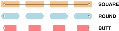
Line appearance can be varied by using PS_LINE_CAP, choosing from SQUARE [Default], ROUND, or BUTT. The circles and thin lines indicate the coordinates. All lines where plotted with the same width and dash-spacing (-W10p,20_20:0).

Here is the source script for the figure above:

gmt begin GMT_cap
	gmt set GMT_THEME cookbook
	cat <<-EOF > butt.txt
	30	50
	170	50
	EOF
	cat <<-EOF > round.txt
	30	70
	170	70
	EOF
	cat <<-EOF > square.txt
	30	90
	170	90
	EOF
	# round
	gmt plot -R0/250/0/100 -Jx1p --PS_LINE_CAP=butt -W10p,lightred,20_20:0 butt.txt
	gmt plot -Wfaint butt.txt
	gmt plot -Sc3p -Gwhite -Wfaint butt.txt
	# miter
	gmt plot --PS_LINE_CAP=round -W10p,lightblue,,20_20:0 round.txt
	gmt plot -Wfaint round.txt
	gmt plot -Sc3p -Gwhite -Wfaint round.txt
	# bevel
	gmt plot --PS_LINE_CAP=square -W10p,lightorange,,20_20:0 square.txt
	gmt plot -Wfaint square.txt
	gmt plot -Sc3p -Gwhite -Wfaint square.txt
	gmt text -F+f8p,Helvetica-Bold+j -Dj5p <<- EOF
	180	50	ML	BUTT
	180	90	ML	SQUARE
	180	70	ML	ROUND
	EOF
gmt end show

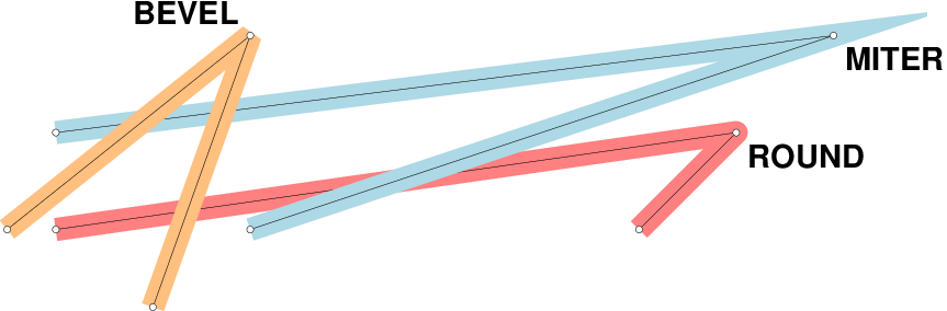
Given lines have finite thickness, there are three types of joints where line-segments meet that can be adjusted with PS_LINE_JOIN. There is BEVEL, ROUND, and MITER. The last setting also depends on PS_MITER_LIMIT which sets a limit on the angle at the mitered joint below which we apply a bevel.

Here is the source script for the figure above:

gmt begin GMT_joint
	gmt set GMT_THEME cookbook
	cat <<-EOF > round.txt
	1	1
	8	2
	7	1
	EOF
	cat <<-EOF > miter.txt
	3 1
	9 3
	1 2
	EOF
	cat <<-EOF > bevel.txt
	0.5	1
	3	3
	2	0.2
	EOF
	# round
	gmt plot -R0/11/0/4 -Jx1.5c --PS_LINE_JOIN=round -W10p,lightred round.txt
	gmt plot -Wfaint round.txt
	gmt plot -Sc3p -Gwhite -Wfaint round.txt
	# miter
	gmt plot --PS_LINE_JOIN=miter --PS_MITER_LIMIT=1 -W10p,lightblue miter.txt
	gmt plot -Wfaint miter.txt
	gmt plot -Sc3p -Gwhite -Wfaint miter.txt
	# bevel
	gmt plot --PS_LINE_JOIN=bevel -W10p,lightorange bevel.txt
	gmt plot -Wfaint bevel.txt
	gmt plot -Sc3p -Gwhite -Wfaint bevel.txt
	gmt text -F+f14p,Helvetica-Bold+j -Dj5p <<- EOF
	3	3	BR	BEVEL
	9	3	TL	MITER
	8	2	TL	ROUND
	EOF
gmt end show

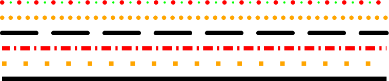
By default, line segments have rectangular ends, but this can change to give rounded ends. When PS_LINE_CAP is set to round then a segment length of zero will appear as a circle. This can be used to create circular dotted lines, and by manipulating the phase shift in the style attribute and plotting the same line twice one can even alternate the color of adjacent items. Figure Line appearance shows various lines made in this fashion by adjusting the joint and cap settings as well as plotting lines twice with different phase offset and color. See the gmt.conf man page for more information.

Line appearance can be varied by using PS_LINE_CAP

Here is the source script for the figure above:

cat << EOF > lines.txt
0       0
5       0
EOF

gmt begin GMT_linecap
	gmt set GMT_THEME cookbook
	gmt plot lines.txt -R-0.25/5.25/-0.2/1.4 -Jx1i -W4p
	gmt plot lines.txt -Y0.2i -W4p,orange,.
	gmt plot lines.txt -Y0.2i -W4p,red,9_4_2_4:2p
	gmt plot lines.txt -Y0.2i -W4p,-  --PS_LINE_CAP=round
	gmt plot lines.txt -Y0.2i -W4p,orange,0_8 --PS_LINE_CAP=round
	gmt plot lines.txt -Y0.2i -W4p,red,0_16  --PS_LINE_CAP=round
	gmt plot lines.txt -W2p,green,0_16:8p  --PS_LINE_CAP=round
gmt end show

Experience has shown that the rendering of lines that are short relative to the pen thickness can sometimes appear wrong or downright ugly. This is a feature of PostScript interpreters, such as Ghostscript. By default, lines are rendered using a fast algorithm which is susceptible to errors for thick lines. The solution is to select a more accurate algorithm to render the lines exactly as intended. This can be accomplished by using the GMT Defaults PS_LINE_CAP and PS_LINE_JOIN by setting both to round. Figure Line appearance displays the difference in results.

Very thick line appearance using the default (left) and round line cap and join (right). The red line (1p width) illustrates the extent of the input coordinates.

Here is the source script for the figure above:

cat > gc.d << END
-82 85
-8  85
END
gmt begin GMT_fatline
	gmt set GMT_THEME cookbook
	gmt plot -R-90/82/0/87+r -JM-45/84.5/2.5i -W30p gc.d
	gmt plot -W1p,red gc.d
	gmt plot -X3.25i -W30p gc.d --PS_LINE_CAP=round --PS_LINE_JOIN=round
	gmt plot -W1p,red gc.d
gmt end show

3.15. Specifying line attributes

A line is drawn with the texture provided by the chosen pen (Specifying pen attributes). However, depending on the module, a line also may have other attributes that can be changed in some modules. Given as modifiers to a pen specification, one or more modifiers may be appended to a pen specification. The line attribute modifiers are:

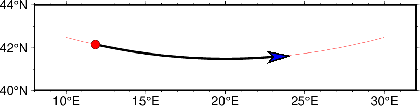
• +ooffset

  Lines are normally drawn from the beginning to the end point. You can modify this behavior by requesting a gap between these terminal points and the start and end of the visible line. Do this by specifying the desired offset between the terminal point and the start of the visible line. Unless you are giving distances in Cartesian data units, please append the distance unit, u. Depending on your desired effect, you can append plot distance units (i.e., cm, inch, point; Section Dimension units)) or map distance units, such as km, degrees, and many other standard distance units listed in Section GMT units. If only one offset is given then it applies equally to both ends of the line. Give two slash-separated distances to indicate different offsets at the beginning and end of the line (and use 0 to indicate no offset at one end).

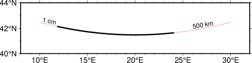
The thin red line shows an original line segment, whereas the 2-point thick pen illustrates the effect of plotting the same line while requesting offsets of 1 cm at the beginning and 500 km at the end, via -W2p+o1c/500k.

Here is the source script for the figure above:

gmt math -T10/30/1 T 20 SUB 10 DIV 2 POW 41.5 ADD = line.txt

gmt begin GMT_lineoffset
	gmt set GMT_THEME cookbook
	gmt plot line.txt -R8/32/40/44 -JM5i -Wfaint,red -Bxaf -Bya2f1 -BWSne --MAP_FRAME_TYPE=plain
	gmt plot line.txt -W2p+o1c/500k
	gmt text -F+f10p+jCM+a << EOF
11.0 42.6 -11.5 1 cm
27.1 42.3 +9.5 500 km
EOF
gmt end show

• +s

  Normally, all PostScript line drawing is implemented as a linear spline, i.e., we simply draw straight line-segments between the map-projected data points. Use this modifier to render the line using Bezier splines for a smoother curve. Note: The spline is fit to the projected 2-D coordinates, not the raw user coordinates (i.e., it is not a spherical surface spline).

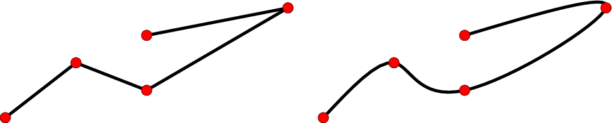
(left) Normal plotting of line given input points (red circles) via -W2p. (right) Letting the projected points be interpolated by a Bezier cubic spline via -W2p+s.

Here is the source script for the figure above:

cat << EOF > line.txt
0       0
1	1
2	0.5
4	2
2	1.5
EOF

gmt begin GMT_bezier
	gmt set GMT_THEME cookbook
	gmt plot line.txt -R-0.25/4.25/-0.2/2.2 -JX3i/1.25i -W2p
	gmt plot line.txt -Sc0.1i -Gred -Wfaint
	gmt plot line.txt -W2p+s -X3i
	gmt plot line.txt -Sc0.1i -Gred -Wfaint
gmt end show

• +v[b|e]vspecs

  By default, lines are normally drawn from start to end. Using the +v modifier you can place arrow-heads pointing outward at one (or both) ends of the line. Use +v if you want the same vector attributes for both ends, or use +vb and +ve to specify a vector only at the beginning or end of the line, respectively. Finally, these two modifiers may both be given to specify different attributes for the two vectors. The vector specification is very rich and you may place other symbols, such as circle, square, or a terminal cross-line, in lieu of the vector head (see plot for more details).

Same line as above but now we have requested a blue vector head at the end of the line and a red circle at the beginning of the line with -W2p+o1c/500k+vb0.2i+gred+pfaint+bc+ve0.3i+gblue. Note that we also prescribed the line offsets in addition to the symbol endings.

Here is the source script for the figure above:

gmt math -T10/30/1 T 20 SUB 10 DIV 2 POW 41.5 ADD = line.txt

gmt begin GMT_linearrow
	gmt set GMT_THEME cookbook
	gmt plot line.txt -R8/32/40/44 -JM5i -Wfaint,red -Bxaf -Bya2f1 -BWSne --MAP_FRAME_TYPE=plain
	gmt plot line.txt -W2p+o1c/500k+vb0.2i+gred+pfaint+bc+ve0.3i+gblue+h0.5
gmt end show

3.16. Specifying area fill attributes

Many plotting programs will allow the user to draw filled polygons or symbols. The fill specification may take two forms (note: not all modules use -G for this task and some have several options specifying different fills):

-Gfill

In the first case we may specify a gray shade (0–255), RGB color (r/g/b all in the 0–255 range or in hexadecimal #rrggbb), HSV color (hue-saturation-value in the 0–360, 0–1, 0–1 range), CMYK color (cyan/magenta/yellow/black, each ranging from 0–100%), or a valid color name; in that respect it is similar to specifying the pen color settings (see pen color discussion under Section Specifying pen attributes).

-GP|ppattern[+bcolor][+fcolor][+rdpi]

The second form allows us to use a predefined bit-image pattern. pattern can either be a number in the range 1–90 or the name of a 1-, 8-, or 24-bit image raster file. The former will result in one of the 90 predefined 64 x 64 bit-patterns provided with GMT and reproduced in Chapter Predefined Bit and Hachure Patterns in GMT. The latter allows the user to create customized, repeating images using image raster files. The optional +rdpi modifier sets the resolution of this image on the page; the area fill is thus made up of a series of these “tiles”. The default resolution is 1200. By specifying upper case -GP instead of -Gp the image will be bit-reversed, i.e., white and black areas will be interchanged (only applies to 1-bit images or predefined bit-image patterns). For these patterns and other 1-bit images one may specify alternative background and foreground colors (by appending +bcolor and/or +fcolor) that will replace the default white and black pixels, respectively. Excluding color from a fore- or background specification yields a transparent image where only the back- or foreground pixels will be painted.

Due to PostScript implementation limitations the raster images used with -G must be less than 146 x 146 pixels in size; for larger images see image. The format of Sun raster files [18] is outlined in Chapter GMT File Formats; other image formats can be used as well. Note that under PostScript Level 1 the patterns are filled by using the polygon as a clip path. Complex clip paths may require more memory than the PostScript interpreter has been assigned. There is therefore the possibility that some PostScript interpreters (especially those supplied with older laserwriters) will run out of memory and abort. Should that occur we recommend that you use a regular gray-shade fill instead of the patterns. Installing more memory in your printer may or may not solve the problem!

Table fillex contains a few examples of fill specifications.

-G128	Solid gray
-G127/255/0	Chartreuse, R/G/B-style
-G#00ff00	Green, hexadecimal RGB code
-G25-0.86-0.82	Chocolate, h-s-v-style
-GDarkOliveGreen1	One of the named colors
-Gp7+r300	Simple diagonal hachure pattern in b/w at 300 dpi
-Gp7+bred+r300	Same, but with red lines on white
-Gp7+bred+f-+r300	Now the gaps between red lines are transparent
-Gpmarble.ras+r100	Using user image of marble as the fill at 100 dpi

3.17. Specifying Fonts

The fonts used by GMT are typically set indirectly via the GMT defaults parameters. However, some programs, like text may wish to have this information passed directly. A font is specified by a comma-delimited attribute list of size, fonttype and fill, each of which is optional. The size is the font size (usually in points) but c, i or p can be added to indicate a specific unit. The fonttype is the name (case sensitive!) of the font or its equivalent numerical ID (e.g., Helvetica-Bold or 1). The fill specifies the gray shade, color or pattern of the text (see section Specifying area fill attributes above). Optionally, you may append =pen to the fill value in order to draw a text outline. If you want to avoid that the outline partially obscures the text, append =~pen instead; in that case only half the linewidth is plotted on the outside of the font only. If an outline is requested, you may optionally skip the text fill by setting it to -, in which case the full pen width is always used. If any of the font attributes is omitted their default or previous setting will be retained. See Chapter PostScript Fonts Used by GMT for a list of all fonts recognized by GMT.

3.18. Stroke, Fill and Font Transparency

The PostScript language has no built-in mechanism for transparency. However, PostScript extensions make it possible to request transparency, and tools that can render such extensions will produce transparency effects. We specify transparency in percent: 0 is opaque [Default] while 100 is fully transparent (i.e., the feature will be invisible). As noted in section Layer transparency: The -t option, we can control transparency on a layer-by-layer basis using the -t option. However, we may also set transparency as an attribute of stroke or fill (including for fonts) settings. Here, transparency is requested by appending @transparency to colors or pattern fills. The transparency mode can be changed by using the GMT default parameter PS_TRANSPARENCY; the default is Normal but you can choose among Color, ColorBurn, ColorDodge, Darken, Difference, Exclusion, HardLight, Hue, Lighten, Luminosity, Multiply, Normal, Overlay, Saturation, SoftLight, and Screen. For more information, see for instance (search online for) the Adobe pdfmark Reference Manual. Most printers and many PostScript viewers can neither print nor show transparency. They will simply ignore your attempt to create transparency and will plot any material as opaque. Ghostscript and its derivatives such as GMT’s psconvert support transparency (if compiled with the correct build option). Note: If you use Acrobat Distiller to create a PDF file you must first change some settings to make transparency effective: change the parameter /AllowTransparency to true in your *.joboptions file.

3.19. Placement of text

Many text labels placed on maps are part of the standard basemap machinery (e.g., annotations, axis labels, plot titles) and GMT automatically takes care of where these are placed and how they are justified. However, when you wish to add extra text to a plot in locations of your choice you will need to understand how we reference text to locations on the map. Figure Text justification discusses the various ways to do this.

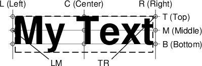
Text strings are placed on maps by associating an anchor point on the string with a reference point on the map. Nine anchor points relative to any text string may be specified by combining any of three letter codes for horizontal (Left, Center, Right) and vertical (Top, Middle, Bottom) alignments.

Here is the source script for the figure above:

gmt begin GMT_pstext_justify
gmt set GMT_THEME cookbook
B=0.2
M=0.38
T=0.56
L=0.10
C=1.04
R=1.98
gmt text -R0/3/0/1.5 -Jx1i -N -C0 -Wthin,- -F+f36p,Helvetica-Bold+jLB << EOF
0.1	0.2	My Text
EOF
gmt plot -N << EOF
>
0.05	$B
2.04	$B
>
0.05	$M
2.04	$M
>
0.05	$T
2.04	$T
>
$L	0
$L	0.65
>
$C	0
$C	0.65
>
$R	0
$R	0.65
EOF
gmt plot -N -Wthinner << EOF
>
0.7	-0.1
$L	$M
>
1.3	-0.1
$R	$T
EOF
gmt text -N -F+f8p+j << EOF
$L	0.69	CB	L (Left)
$C	0.69	CB	C (Center)
$R	0.69	CB	R (Right)
2.07	$T	LM	T (Top)
2.07	$M	LM	M (Middle)
2.07	$B	LM	B (Bottom)
0.6	-0.05	LM	LM
1.37	-0.05	RM	TR
EOF
gmt plot -Sc0.05 << EOF
$L	$B
$L	$M
$L	$T
$C	$B
$C	$M
$C	$T
$R	$B
$R	$M
$R	$T
EOF
gmt end show

Notice how the anchor points refers to the text baseline and do not change for text whose letters extend below the baseline.

The concept of anchor points extends to entire text paragraphs that you may want to typeset with text.

A related point involves the footprint of the text and any background panel on the map. We determine the bounding box for any text string, but very often we wish to extend this box outwards to allow for some clearance between the text and the space surrounding it. Programs that allows for such clearance will let you specify offsets dx and dy that is used to enlarge the bounding box, as illustrated in Figure Text clearance.

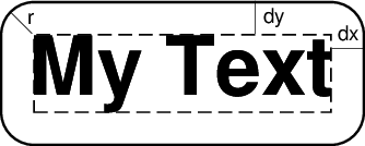
The bounding box of any text string can be enlarged by specifying the adjustments dx and dy in the horizontal and vertical dimension. The shape of the bounding box can be modified as well, including rounded or convex rectangles. Here we have chosen a rounded rectangle, requiring the additional specification of a corner radius, r.

Here is the source script for the figure above:

gmt begin GMT_pstext_clearance
gmt set GMT_THEME cookbook
gmt text -R0/3/-0.1/1.5 -Jx1i -C0.2i+tO -Wthick -F+f36p,Helvetica-Bold << EOF
1.5	0.5	My Text
EOF
gmt text -C0 -Wthin,- -F+f36p,Helvetica-Bold << EOF
1.5	0.5	My Text
EOF
gmt text -F+f9p+j << EOF
2.00	0.80	LM	dy
2.52	0.65	CB	dx
0.56	0.75	LB	r
EOF
gmt plot << EOF
>
1.95	0.69
1.95	0.89
>
2.42	0.60
2.62	0.60
>
0.59	0.69
0.46	0.82
EOF
gmt end show

3.20. Color palette tables

Several programs need to relate user data to colors, shades, or even patterns. For instance, programs that read 2-D gridded data sets and create colored images or shaded reliefs need to be told what colors to use and over what z-range each color applies. Other programs may need to associate a user value with a color to be applied to a symbol, line, or polygon. This is the purpose of the color palette table (CPT). For most applications, you will simply create a CPT using the tool makecpt which will take an existing dynamic master color table and stretch it to fit your chosen data range, or use grd2cpt to build a CPT based on the data distribution in one or more given grid files. However, in rare situations you may need to make a CPT by hand or using text tools like awk or perl. Finally, if you have your own preferred color table you can convert it into a dynamic CPT and place it in your GMT user directory and it will be found and behave like other GMT master CPTs.

Color palette tables (CPT) comes in two flavors: (1) Those designed to work with categorical data (e.g., data where interpolation of values is undefined) and (2) those designed for regular, continuously-varying data. In both cases the fill information follows the format given in Section Specifying area fill attributes. The z-values in CPTs can be scaled by using the +u|Uunit mechanism. Append these modifiers to your CPT names when used in GMT commands. The +uunit modifier will scale z from unit to meters, while +Uunit does the inverse (scale z from meters to unit).

Note: Users are allowed to name their CPT files anything they want, but we recommend the use of the file extension “.cpt”. This allows us to prevent any confusion when parsing filenames that may have sequences that otherwise might look like a file modifier (e.g., data.my+u5.cpt). Since valid modifiers are appended to a file name, finding such an extension simplifies parsing.

Since GMT supports several coordinate systems for color specification, many master (or user) CPTs will contain the special comment

# COLOR_MODEL = model

where model specifies how the color-values in the CPT should be interpreted. By default we assume colors are given as red/green/blue triplets (each in the 0-255 range) separated by slashes (model = rgb), but alternative representations are the HSV system of specifying hue-saturation-value triplets (with hue in 0-360 range and saturation and value ranging from 0-1) separated by hyphens (model = hsv), or the CMYK system of specifying cyan/magenta/yellow/black quadruples in percent, separated by slashes (model = cmyk).

3.20.1. Categorical CPTs

Categorical data are information on which normal numerical operations are not defined. As an example, consider various land classifications (desert, forest, glacier, etc.) and it is clear that even if we assigned a numerical value to these categories (e.g., desert = 1, forest = 2, etc) it would be meaningless to compute average values (what would 1.5 mean?). For such data a special format of the CPTs are provided. Here, each category is assigned a unique key, a color or pattern, and an optional label (usually the category name) marked by a leading semi-colon. Keys (if numerical) must be monotonically increasing but do not need to be consecutive. The format is

key1	Fill	[;label]
…
keyn	Fill	[;label]

For usage with points, lines, and polygons, the keys may be text (single words), and then GMT will use strings to find the corresponding Fill value. Strings may be supplied as trailing text in data files (for points) or via the -Zcategory option in multiple segment headers (or set via -aZ=aspatialname). If any of your keys are called B, F, or N you must escape them with a leading backslash to avoid confusion with the flags for background, foreground and NaN colors. The Fill information follows the format given in Section Specifying area fill attributes. For categorical data, background color or foreground color do not apply. The not-a-number (NaN) color (for key-values not found or blank) is defined in the gmt.conf file, but it can be overridden by the statement

N

Fillnan

While you can make such categorical CPTs by hand, both makecpt and grd2cpt have options to simplify adding string keys and labels from comma-separated arguments.

3.20.2. Regular CPTs

Suitable for continuous data types and allowing for color interpolations, the format of the regular CPTs is:

z0	Colormin	z1	Colormax	[A]	[;label]
…
zn-2	Colormin	zn-1	Colormax	[A]	[;labell[;labelu]]

Thus, for each “z-slice”, defined as the interval between two boundaries (e.g., \(z_0\) to \(z_1\)), the color can be constant (by letting Color\(_{max}\) = Color\(_{min}\) or -) or a continuous, linear function of z. If patterns are used then the second (max) pattern must be set to -. The optional flag A is used to indicate annotation of the color scale when plotted using colorbar. The optional flag A may be L, U, or B to select annotation of the lower, upper, or both limits of the particular z-slice, respectively. However, the standard -B option can be used by colorbar to affect annotation and ticking of color scales. Just as other GMT programs, the stride can be omitted to determine the annotation and tick interval automatically (e.g., -Baf). The optional semicolon followed by a text label will make colorbar, when used with the -L option, place the supplied label instead of formatted z-values. Note: If the last slice should have both lower and upper custom labels then you must supply two semicolon-separated labels and set the annotation code to B.

The background color (for z-values < \(z_0\)), foreground color (for z-values > \(z_{n-1}\)), and not-a-number (NaN) color (for z-values = NaN) are all defined in the gmt.conf file, but can be overridden by the statements

B	Fillback
F	Fillfore
N	Fillnan

which can be inserted into the beginning or end of the CPT. If you prefer the HSV system, set the gmt.conf parameter accordingly and replace red, green, blue with hue, saturation, value. Color palette tables that contain gray-shades only may replace the r/g/b triplets with a single gray-shade in the 0–255 range. For CMYK, give c/m/y/k values in the 0–100 range.

A few programs (i.e., those that plot polygons such as grdview, colorbar, plot and plot3d) can accept pattern fills instead of gray-shades. You must specify the pattern as in Section Specifying area fill attributes (no leading -G of course), and only the first pattern (for low z) is used (we cannot interpolate between patterns). Finally, some programs let you skip features whose z-slice in the CPT file has gray-shades set to -. As an example, consider

30	p16+r200	80	-
80	-	100	-
100	200/0/0	200	255/255/0
200	yellow	300	green

where slice 30 < z < 80 is painted with pattern # 16 at 200 dpi, slice 80 < z < 100 is skipped, slice 100 < z < 200 is painted in a range of dark red to yellow, whereas the slice 200 < z < 300 will linearly yield colors from yellow to green, depending on the actual value of z.

Some programs like grdimage and grdview apply artificial illumination to achieve shaded relief maps. This is typically done by finding the directional gradient in the direction of the artificial light source and scaling the gradients to have approximately a normal distribution on the interval [-1,+1]. These intensities are used to add “white” or “black” to the color as defined by the z-values and the CPT. An intensity of zero leaves the color unchanged. Higher values will brighten the color, lower values will darken it, all without changing the original hue of the color (see Chapter Color Systems and Artificial Illumination for more details). The illumination is decoupled from the data grid file in that a separate grid file holding intensities in the [-1,+1] range must be provided. Such intensity files can be derived from the data grid using grdgradient and modified with grdhisteq, but could equally well be a separate data set. E.g., some side-scan sonar systems collect both bathymetry and backscatter intensities, and one may want to use the latter information to specify the illumination of the colors defined by the former. Similarly, one could portray magnetic anomalies superimposed on topography by using the former for colors and the latter for shading.

3.20.3. Master (dynamic) CPTs

The CPTs distributed with GMT are dynamic. This means they have several special properties that modify the behavior of programs that use them. Dynamic CPTs comes in a few different flavors: Some CPTs were designed to behave differently across a hinge value (e.g., a CPT designed specifically for topographic relief may include a discontinuity in color across the coastline at z = 0), and when users select these CPTs they will be stretched to fit the user’s desired data range separately for each side of this hard hinge. Basically, a hard hinge CPT is the juxtaposition of two different CPTs joined at the hinge and these sections are stretched independently. Such CPT files are identified as such via the special comment

# HARD_HINGE

and all hard hinges occur at data value z = 0 (but you can change this value by adding +hvalue to the name of the CPT). Other CPTs may instead have a soft hinge which indicates a natural hinge or transition point in the CPT itself, unrelated to any natural data set per se. These CPTs are flagged by the special comment

# SOFT_HINGE

CPTs with soft hinges behave as regular (non-hinge) CPTs unless the user activates then by appending +h[hinge] to the CPT name. This modifier will convert the soft hinge into a hard hinge at the user-specified data value hinge [which defaults to 0]. Note that if your specified data range excludes an activated soft or hard hinge then we only perform color sampling from the half of the CPT that pertains to the data range. All dynamic CPTs will need to be stretched to the user’s preferred range, and there are two modes of such scaling: Some CPTs designed for a specific application (again, the topographic relief is a good example) have a default range specified in the master table via the special comment

# RANGE = <zmin/zmax>

and when used by applications the CPT may be automatically stretched to reflect this natural range. In contrast, dynamic CPTs without a natural range are instead stretched to fit the range of the data in question (e.g., a grid’s range). Exceptions to these rules are implemented in the two CPT-producing modules makecpt and grd2cpt, both of which can read dynamic CPTs and produce static CPTs satisfying a user’s specific range needs. These tools can also read static CPTs for which a new range must be specified (or computed from data), reversing the order of colors, and even isolating a section of an incoming CPT. Here, makecpt can be told the data range or compute it from data tables while grd2cpt can derive the range from one or more grids.

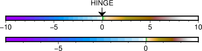
The top color bar is a dynamic master CPT (here, globe) with a hard hinge at sea level and a natural range from -10,000 to +10,000 meters. However, our data range is asymmetrical, going from -8,000 meter depths up to +3,000 meter elevations. Because of the hinge, the two sides of the CPT will be stretched separately to honor the desired range while utilizing the full color range.

Here is the source script for the figure above:

gmt begin GMT_hinge
	gmt set GMT_THEME cookbook
	gmt makecpt -Cglobe -T-8000/3000
	gmt colorbar -B -Dx0/0+w4.5i/0.1i+h -W0.001
	gmt colorbar -Cglobe -B -Dx0/0+w4.5i/0.1i+h -W0.001 -Y0.5i
	echo 2.25 0.1 90 0.2i | gmt plot -R0/4.5/0/1 -Jx1i -Sv0.1i+a80+b -W1p -Gblack
	gmt text -F+f12p+jCB <<- EOF
	2.25	0.35	HINGE
	EOF
gmt end show

All CPT master tables can be found in Chapter Of Colors and Color Legends where those with hard or soft hinges are identified by triangles at their hinges.

3.20.4. CPTs from color lists

GMT can build color tables “on the fly” from a comma-separated list of colors and a range of z-values to go with them. As illustrated below, there are four different ways to create such CPTs. In this example, we will operate with a list of three colors: red,yellow and purple, given to modules with the option -Cred,yellow,purple, and utilize a fixed data range of z = 0-6. Four different CPTs result because we either select a continuous or discrete table, and because the z-intervals are either equidistant or arbitrary. The top continuous color table with equidistant spacing (a) is selected with the range -T0/6, meaning the colors will continuously change from red (at z = 0) via yellow (at z = 3) to purple (at z = 6). Next, a discrete table with the same range (b) is obtained with -T0/6/2, yielding colors that are either constant red (z = 0-2), yellow (z = 2-4) or purple (z = 4-6). The next discrete table (c) illustrates how to specify arbitrary node points in the CPT by providing a comma-separated list of values (-T0,4,5.5,6). Now, the constant color intervals have unequal ranges, illustrated by red (z = 0-4), yellow (z = 4-5.5) and purple (z = 5.5-6). Finally, we create a continuous color table (d) with arbitrary nodes by giving -T0,2,6 and adding -Z; the latter option forces a continuous CPT pinned to a given list of node values. Now, the colors continuously change from red (at z = 0) via yellow (at z = 2) to purple (at z = 6). Modules that obtain the z-range indirectly (e.g., grdimage) may use the exact data range to set the quivalent of a -Tmin/max option. You may append +idz to the color list to have the min and max values rounded down and up to nearest multiple of dz, respectively.

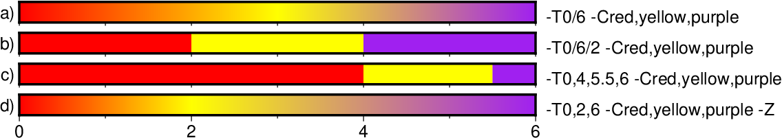
Lists of colors (here red,yellow,purple) can be turned into discrete or continuous CPT tables on the fly.

Here is the source script for the figure above:

gmt begin GMT_colorlist
	gmt set GMT_THEME cookbook
	gmt makecpt -T0,2,6 -Cred,yellow,purple -Z
	gmt colorbar -R0/4/0/4 -Jx1i -C -Bx -By+l"d)" -Dx0/0+w5i/0.2i+h+mu
	echo "5.1 0 -T0,2,6 -Cred,yellow,purple -Z" | gmt text -F+f12p+jLB -N
	gmt makecpt -T0,4,5.5,6 -Cred,yellow,purple
	gmt colorbar -C -Bxf1 -By+l"c)" -Dx0/0+w5i/0.2i+h+mu -Y0.3i
	echo "5.1 0 -T0,4,5.5,6 -Cred,yellow,purple" | gmt text -F+f12p+jLB -N
	gmt makecpt -T0/6/2 -Cred,yellow,purple
	gmt colorbar -C -Bxf1 -By+l"b)" -Dx0/0+w5i/0.2i+h+mu -Y0.3i
	echo "5.1 0 -T0/6/2 -Cred,yellow,purple" | gmt text -F+f12p+jLB -N
	gmt makecpt -T0/6 -Cred,yellow,purple
	gmt colorbar -C -Bxf1 -By+l"a)" -Dx0/0+w5i/0.2i+h+mu -Y0.3i
	echo "5.1 0 -T0/6 -Cred,yellow,purple" | gmt text -F+f12p+jLB -N
gmt end show

3.20.5. Cyclic (wrapped) CPTs

Any color table you produce can be turned into a cyclic or wrapped color table. This is performed by adding the -Ww option when running makecpt or grd2cpt. This option simply adds the special comment

# CYCLIC

to the color table and then GMT knows that when looking up a color from a z value it will remove an integer multiple of the z-range represented by the color table so that we are always inside the range of the color table. This means that the fore- and back-ground colors can never be activated. Wrapped color tables are useful for highlighting small changes.

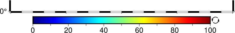
Cyclic color bars are indicated by a cycle symbol on the left side of the bar.

Here is the source script for the figure above:

gmt begin GMT_cyclic
	gmt set GMT_THEME cookbook
	gmt makecpt -T0/100 -Cjet -Ww
	gmt basemap -R0/20/0/1 -JM5i -BWse -B
	gmt colorbar -C -B -DJBC
gmt end show

3.20.6. Manipulating CPTs

There are many ways to turn a master CPT into a custom CPT that works for your particular data range. The tools makecpt and grd2cpt allow several types of transformations to take place:

1. You can reverse the z-direction of the CPT using option -Iz. This is useful when your data use a different convention for positive and negative (e.g., perhaps using positive depths instead of negative relief).

2. You can invert the order of the colors in the CPT using option -Ic. This is different from the previous option in that only the colors are rearranged (it is also possible to issue -Icz to combine both effects.)

3. You can select just a subset of a master CPT with -G, in effect creating a modified master CPT that can be scaled further.

4. Finally, you can scale and translate the (modified) master CPT range to your actual data range or a sub-range thereof.

The order of these transformations is important. For instance, if -Iz is given then all other z-values need to be referred to the new sign convention. For most applications only the last transformation is needed.

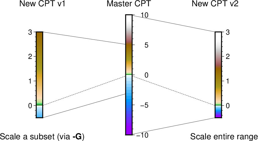
Examples of two user CPTs for the range -0.5 to 3 created from the same master. One (left) extracted a subset of the master before scaling while the other (right) used the entire range.

Here is the source script for the figure above:

gmt begin GMT_CPTscale
	gmt set GMT_THEME cookbook
	gmt plot -R0/6/0/6 -Jx1i -W0.25p << EOF
> Normal scaling of whole CPT
3	2.9
5	2.5
>
3	0.1
5	0.5
> Truncated with -G
3	2.2
1	2.5
>
3	1.08
1	0.5
> Dash the hinges -W0.25p,-
1	0.785
3	1.5
>
3	1.5
5	0.785
EOF
	gmt colorbar -Cglobe -B -Dx3i/1.5i+w2.8i/0.15i+jCM -W0.001
	gmt makecpt -Cglobe -T-500/3000
	gmt colorbar -C -B -Dx5i/1.5i+w2.0i/0.15i+jLM -W0.001
	gmt makecpt -Cglobe -G-3000/5000 -T-500/3000
	gmt colorbar -C -B -Dx1i/1.5i+w2.0i/0.15i+jRM+ma -W0.001
	gmt text -N -F+f14p+j << EOF
0	0	LB	Scale a subset (via @%1%-G@%%)
6	0	RB	Scale entire range
3	3.1	CB	Master CPT
1	3.1	CB	New CPT v1
5	3.1	CB	New CPT v2
EOF
gmt end show

3.20.7. Automatic CPTs

A few modules (grdimage, grdview) that expects a CPT option will provide a default CPT if none is provided. By default, the default CPT is the turbo color table, but this is overridden if the user uses the @earth_relief (we select geo) or @srtm_relief (we select srtm) data sets. After selection, these CPTs are read and scaled to match the range of the grid values. You may append +idz to the CPT to have the exact range rounded to nearest multiple of dz. This is helpful if you plan to place a colorbar and prefer start and stop z-values that are multiples of dz.

3.21. The Drawing of Vectors

GMT supports plotting vectors in various forms. A vector is one of many symbols that may be plotted by plot and plot3d, is the main feature in grdvector, and is indirectly used by other programs. All vectors plotted by GMT consist of two separate parts: The vector line (controlled by the chosen pen attributes) and the optional vector head(s) (controlled by the chosen fill). We distinguish between three types of vectors:

1. Cartesian vectors are plotted as straight lines. They can be specified by a start point and the direction and length (in map units) of the vector, or by its beginning and end point. They may also be specified giving the azimuth and length (in km) instead.

2. Circular vectors are (as the name implies) drawn as circular arcs and can be used to indicate opening angles. It accepts an origin, a radius, and the beginning and end angles.

3. Geo-vectors are drawn using great circle arcs. They are specified by a beginning point and the azimuth and length (in km) of the vector, or by its beginning and end point.

Examples of Cartesian (left), circular (middle), and geo-vectors (right) for different attribute specifications. Note that both full and half arrow-heads can be specified, as well as no head at all.

Here is the source script for the figure above:

gmt begin GMT_arrows
gmt set GMT_THEME cookbook
	gmt plot -R0/5/0/5 -JX1.75i -S -W1.5p -Gred -B0 --MAP_VECTOR_SHAPE=0.5 << EOF
0.5	0.5	4.5	0.5	v0.2i+s
0.5	1.5	4.5	1.5	v0.2i+s+e
0.5	2.5	4.5	2.5	v0.2i+s+b+er
0.5	3.5	4.5	3.5	v0.2i+s+b+e
0.5	4.5	4.5	4.5	v0.2i+s+el
EOF
	gmt plot -S -W1.5p -Gred -B0 --MAP_VECTOR_SHAPE=0.5 -X2i << EOF
0.5	0.5	1.5	0	90	m0.2i
0.5	0.5	1.3	0	90	m0.2i+e
0.5	0.5	1.1	0	90	m0.2i+b
0.5	0.5	0.9	0	90	m0.2i+b+el
0.5	0.5	0.7	0	90	m0.2i+r+e
0.5	0.5	0.3	0	90	M0.2i+r+e
EOF
	gmt plot -R0/90/-41.17/41.17 -JM1.75i -S -W1.5p -Gred -B0 --MAP_VECTOR_SHAPE=0.5 -X2i --MAP_FRAME_TYPE=plain << EOF
10	0	90	8000	=0.2i
10	13	90	8000	=0.2i+e
10	-13	90	8000	=0.2i+b
10	25	90	8000	=0.2i+b+e
10	-25	90	8000	=0.2i+b+er
10	35	90	8000	=0.2i+r+b
10	-35	90	8000	=0.2i+bl
EOF
gmt end show

There are numerous attributes you can modify, including how the vector should be justified relative to the given point (beginning, center, or end), where heads (if any) should be placed, if the head should just be the left or right half, if the vector attributes should shrink for vectors whose length are less than a given cutoff length, and the size and shape of the head. These attributes are detailed further in the relevant manual pages.

Examples of different vector heads and attributes. The default is the standard triangular arrow head, which can be modified by adjusting the apex angle [30] or changing its shape via the MAP_VECTOR_SHAPE setting. Other vector heads are the circle (c), the terminal line (t), the arrow fin (i) and the plain head (A) and tail (I); the last two are line-drawings only and cannot be filled.

Here is the source script for the figure above:

gmt begin GMT_arrows_types
gmt set GMT_THEME cookbook
	gmt plot -R0/10/0/7 -JX5.75i/1.75i -S -W1.5p -Gred -B0 --MAP_VECTOR_SHAPE=0 << EOF
0.5	0.5	4.5	0.5	v0.25i+s+e+a40
0.5	1.5	4.5	1.5	v0.25i+s+b
0.5	2.5	4.5	2.5	v0.25i+s+e+b
EOF
	gmt plot -S -W1.5p -Gred --MAP_VECTOR_SHAPE=0.5 << EOF
0.5	3.5	4.5	3.5	v0.25i+s+e+b
0.5	4.5	4.5	4.5	v0.25i+s+b+a45
0.5	5.5	4.5	5.5	v0.25i+s+e+bi
0.9	6.5	4.1	6.5	v0.25i+s+eI+bI
EOF
	gmt plot -S -W1.5p -Gred -X2.875i << EOF
0.5	0.5	4.5	0.5	v0.25i+s+et
0.5	1.5	4.5	1.5	v0.25i+s+bc
0.5	2.5	4.5	2.5	v0.25i+s+et+bt
EOF
	gmt plot -S -W1.5p -Gred --MAP_VECTOR_SHAPE=0.5 << EOF
0.5	3.5	4.5	3.5	v0.25i+s+e+bt
0.5	4.5	4.5	4.5	v0.25i+s+b+ec+a45
EOF
	gmt plot -S -W1.5p -Gred --MAP_VECTOR_SHAPE=0.5 << EOF
0.5	5.5	4.5	5.5	v0.25i+s+b+ei
0.5	6.5	4.5	6.5	v0.25i+s+bA+eA
EOF
gmt end show

3.22. Character escape sequences

For annotation labels or text strings plotted with text, GMT provides several escape sequences that allow the user to temporarily switch to the symbol font, turn on sub- or superscript, etc., within words. These conditions are toggled on/off by the escape sequence @x, where x can be one of several types. The escape sequences recognized in GMT are listed in Table escape. Only one level of sub- or superscript is supported. Note that under Windows the percent symbol indicates a batch variable, hence you must use two percent-signs for each one required in the escape sequence for font switching. In bash scripts the brackets have special meaning, hence you must add double quotes.

@~	Turns symbol font on or off
@+	Turns superscript on or off
@-	Turns subscript on or off
@#	Turns small caps on or off
@_	Turns underline on or off
@%fontno%	Switches to another font; @%% resets to previous font
@:size:	Switches to another font size; @:: resets to previous size
@;color;	Switches to another font color; @;; resets to previous color
@!	Creates one composite character of the next two characters
@.	Prints the degree symbol
@@	Prints the @ sign itself

Shorthand notation for a few special European characters has also been added (for others you must use the full octal code):

Code	Effect	Code	Effect
@E	Æ	@e	æ
@O	Ø	@o	ø
@A	Å	@a	å
@C	Ç	@c	ç
@N	Ñ	@n	ñ
@U	Ü	@u	ü
@s	ß	@i	í

However, if your input text contains UTF-8 code characters (e.g., ü, Î) and you select the ISOLatin1+ character encoding then GMT will substitute the correct PostScript octal codes for you automatically.

PostScript fonts used in GMT may be re-encoded to include several accented characters used in many European languages. To access these, you must specify the full octal code \xxx allowed for your choice of character encodings determined by the PS_CHAR_ENCODING setting described in the gmt.conf man page. Only the special characters belonging to a particular encoding will be available. Many characters not directly available by using single octal codes may be constructed with the composite character mechanism @!.

Some examples of escape sequences and embedded octal codes in GMT strings using the Standard+ encoding:

2@~p@~r@+2@+h@-0@- E\363tv\363s = 2\(\pi r^2h_0\) Eötvös

10@+-3 @Angstr@om = 10\(^{-3}\) Ångstrøm

Stresses are @~s@~@+*@+@-xx@- MPa = Stresses are \(\sigma^{*}_{xx}\) MPa

Se@nor Gar@con = Señor Garçon

M@!\305anoa stra@se = Manoa straße

A@#cceleration@# (ms@+-2@+) = ACCELERATION (ms\(^{-2}\))

The option in text to draw a rectangle surrounding the text will not work for strings with escape sequences. A chart of characters and their octal codes is given in Chapter Chart of Octal Codes for Characters.

3.23. Plot embellishments

Apart from visualizing your data sets, GMT maps can also be embellished in several ways. The 9 embellishments currently available are

• Map scale showing the true scale at some location(s) on the map.

• Directional rose showing true north and other cardinal directions.

• Magnetic rose showing magnetic north and declination deviations.

• Color bar relating the colors of your image to the data values.

• Map legend showing the meaning of the symbols on your map.

• Image overlay of raster images or EPS figures (e.g., institutional logos, photos, etc.).

• GMT logo overlay.

• Map inset showing perhaps the location of your detailed area in a regional or global context.

• Vertical scale showing the vertical scale of anomalies on a map.

Each of these features share a common system for specifying the location on the plot where the feature will be placed. They also share a common way for specifying the placement of a rectangular panel behind the feature (to provide a uniform background, for instance). Thus, before we discuss the different features in more detail we will first review the “reference point/anchor point” system used by GMT to specify such locations in relation to the underlying map, and then discuss the background panel attribute settings.

3.23.1. Reference and anchor point specification

The placement of a map feature (here represented by a green rectangle) in relation to the underlying map. The nine named reference points (blue circles) on the map perimeter (and center) can be used to specify a location. Using the same system of nine points on the map feature (cyan circles) we select one of these as our anchor point (here TL, indicated by the orange square). The anchor point can optionally be shifted away from the reference point by an amount dx/dy in the direction implied by the anchor point (in this case to the top and left), yielding the adjusted anchor point (red square). The feature is then placed such that its adjusted anchor point matches the reference point.

Here is the source script for the figure above:

gmt begin GMT_anchor
	gmt set GMT_THEME cookbook
	gmt basemap -R0/1/0/1 -JX5i/2i -Ba1f0.5 -BwSnE+gbisque
	gmt inset begin -DjTL+o0.7i/0.5i+w1.5i/0.75i -F+glightgreen+p1p
	gmt inset end
	gmt plot -W0.25p,- << EOF
0	0.75
0.14	0.75
0.14	1
EOF
	gmt plot -W2p << EOF
0	1
0.14	0.75
EOF
	echo 0 1 | gmt plot  -Ss0.2i -Gred -W0.25p -N
	echo 0.14 0.75 | gmt plot  -Ss0.2i -Gorange -W0.25p -N
	gmt plot -Sc0.075i -Gblue -W0.25p -N << EOF
0	0
0.5	0
1	0
0	0.5
0.5	0.5
1	0.5
0	1
0.5	1
1	1
EOF
	gmt plot -Sc0.075i -Gcyan -W0.25p -N << EOF
0.14	0.375
0.29	0.375
0.44	0.375
0.14	0.5625
0.29	0.5625
0.44	0.5625
0.14	0.75
0.29	0.75
0.44	0.75
EOF
	gmt text -F+f14p,Helvetica-Bold+j -Dj0.25i+v0.25p -N << EOF
0	0  	RT	LB
0.5	0  	CT	CB
1	0  	LT	RB
0	0.5	RM	LM
0.5	0.5	LM	CM
1	0.5	LM	RM
0	1  	RB	LT
0.5	1  	CB	CT
1	1  	LB	RT
EOF
	echo 0 0.75 0 1 | gmt plot -N -Sv0.2i+bt+et+s -W1p -D-0.2i/0
	echo 0 1 0.14 1 | gmt plot -N -Sv0.2i+bt+et+s -W1p -D0/0.2i
	echo 0.07 1 dx  | gmt text -N -F+f12p,Times-Italic+jCM -Gwhite -D0/0.2i
	echo 0 0.875 dy | gmt text -N -F+f12p,Times-Italic+jCM -Gwhite -D-0.2i/0
gmt end show

Placing a feature on the map means selecting a reference point somewhere on the map, an anchor point somewhere on the feature, and then positioning the feature so that the two points overlap. It may be helpful to consider the analog of a boat dropping an anchor: The boat navigates to the reference point and then, depending on where on the boat the anchor is located, moves so that the anchor connection point overlies the reference point, then drops the anchor. There are four different ways to specify the reference point on a map, allowing for complete freedom to select any location inside or outside the map. The reference point syntax is [g|j|J|n|x]refpoint; the five codes g|j|J|n|x refer to the five ways:

1. [g] Specify refpoint using data coordinates, e.g., the longitude and latitude of the reference point. This mechanism is useful when you want to tie the location of the feature to an actual point best described by data coordinates. An example of such a reference point might be g135W/20N.

1. [j] Specify refpoint using one of the nine justification codes, equivalent to the justification codes for placing text strings in text. This mechanism is illustrated in the figure above and is the preferred mechanism when you just want to place the feature inside the basemap at one of the corners or centered at one of the sides (or even smack in the middle). Justification codes are a combination of a horizontal (L, C, R) and a vertical (T, M, B) code. An example of such a reference point might be jTL. When used, the anchor point on the map feature will default to the same justification, i.e., TL in this example.

2. [J] This is the same as j except it implies that the default anchor point is the mirror opposite of the justification code. Thus, when using JTL, the anchor point on the map feature will default to BR. This is practical for features that are drawn outside of the basemap (like color bars often are).

1. [x] Specify refpoint using plot coordinates, i.e., the distances in inches, centimeters, or points from the lower left plot origin. This mechanism is preferred when you wish to lay out map features using familiar measurements of distance from origins. An example of such a reference point might be x2.75i/2c.

1. [n] Specify refpoint using normalized coordinates, i.e., fractional coordinates between 0 and 1 in both the x and y directions. This mechanism avoids units and is useful if you want to always place features at locations best referenced as fractions of the plot dimensions. An example of such a reference point might be n0.2/0.1.

If no code is specified we default to x.

With the reference point taken care of, it is time to select the anchor point. While the reference point selection gives unlimited flexibility to pick any point inside or outside the map region, the anchor point selection is limited to the nine justification points discussed for the j reference point code above. Add +janchor to indicate which justification point of the map feature should be co-registered with the chosen reference point. If an anchor point is not specified then it defaults to the justification point set for the reference point (if jcode was used to set it), or to the mirror opposite of the reference point (if Jcode was used); with all other specifications of the reference point, the anchor point takes on the default value of MC (for map rose and map scale) or BL (all other map features). Adding +janchor overrules those defaults. For instance, +jTR would select the top right point on the map feature as the anchor.

It is likely that you will wish to offset the anchor point away from your selection by some arbitrary amount, particularly if the reference point is specified with j|Jcode. Do so with +odx[/dy], where dy equals dx if it is not provided. These increments are added to the projected plot coordinates of the anchor point, with positive values moving the reference point in the same direction as the 2-character code of the anchor point implies. Finally, the adjusted anchor point is matched with the reference point.

Take for example an anchor point on the top left of the map feature, either by using a reference point jTL, or JBR, or explicitly setting +jTL. Then +o2c/1c will move the anchor point 2 cm left and 1 cm above the top left corner of the map feature. In other words, the top left corner of the map feature will end up 2 cm to the right and 1 cm below the selected reference point.

Similarly, +jBR will align the bottom right corner of the map feature, and +o2c/1c will offset it 2 cm to the left and 1 cm up. When using middle (M) or center (C) justifications, to offset works the same way as bottom (B) or left (L), respectively, i.e., moving the map feature up or to the right.

3.23.2. The background panel

For most maps you will wish to place a background panel of uniform color behind any of the map features you plan to add. Because the panel is linked to the map feature you have selected, the parameters such as location and dimensions are handled automatically. What remains is to specify the attributes of the panel. Typically, panels settings are given via a module’s -F option by appending one or more modifiers. Here is a list of the attributes that are under your control:

1. Color or pattern. You specify the fill you want with +gfill [Default is no fill]. For instance, paint the panel yellow with +gyellow.

2. Panel frame pen. Turn on the frame outline with +p, using the pen defined via MAP_FRAME_PEN. You may override this choice with +ppen [Default is no outline]. A very bold red outline might look like +pthick,red.

3. Rounded versus straight rectangle. By specifying a corner radius with +rradius you can round the corners [Default is no rounding]. Here is a 0.5-cm radius rounding: +r0.5c.

4. Inner frame. A secondary, inner frame outline may be added as well with the modifier +i[[gap/]pen]. The default pen is given by MAP_DEFAULT_PEN, with a default gap between the outer and inner frames of 2 points. Add arguments to override these defaults, such as +i0.1c/thin,dashed to get a thin, dashed inner frame offset by 0.1 cm from the main (outer) frame.

5. Panel clearance. The panel’s dimensions are automatically determined from knowledge of its contents. However, it is sometimes required to add some extra clearance around most or all sides, and you can do so with +c[clearance], with a 4-point clearance being the default. Add one (uniform), two (different horizontal and vertical clearances), or four (separate for sides west, east, south, and north) clearances, separated by slashes. For instance, to add a 1 cm clearance in x and 5 points in y, use +c1c/5p.

6. Drop-down shadow. Append +s to simulate a gray shadow cast toward the southeast. You may append [dx/dy/][shade] to change the shade color and the offset of the shade [Default is 4p/-4p/gray50]. If happy with the placement but desiring a dark blue shadow, add +sdarkblue.

A map panel is a rectangular background placed behind any of the map features. It has several attributes that can be changed with panel option modifiers. The light green rounded rectangle was specified with -F+glightgreen+r, while the white panel on the lower right was set with -F+p1p+i+s+gwhite+c0.1i (we added a light dashed box to indicate the effect of the clearance setting).

Here is the source script for the figure above:

gmt begin GMT_panel
	gmt set GMT_THEME cookbook
	gmt basemap -R0/2/0/1 -JX5i/2i -B0
	gmt inset begin -DjTL+o0.2i+w1.75i/0.75i -F+glightgreen+r
	gmt inset end
	gmt inset begin -DjBR+o0.3i+w1.75i/0.75i -F+p1p+i+s+gwhite+c0.1i
	gmt inset end
	gmt inset begin -DjBR+o0.3i+w1.75i/0.75i -F+p0.25p,-+c0
	gmt inset end
gmt end show

3.23.3. Placing map scales

Traditionally, a map scale is added to maps for helping the reader understand the particular scale used for this map, i.e., it portrays the relationship between actual distances on the Earth (in km, miles, meters, etc.) and distances on the map (in cm, inches, points). Depending on the map projection the map scale will vary continuously but may be constant along a line of latitude (e.g., Mercator projection). Thus, in placing the map scale on the map there are two locations involved: (1) The reference point where the map scale’s anchor should be pinned, and (2) the projection point where the scale is computed and thus where the map scale is true. Map scales can be plotted by basemap or coast, and in addition to the the required refpoint and anchor arguments specifying where the scale should be placed there are both required and optional modifiers. These are given via these modules’ -L option. Here is a list of the attributes that is under your control:

1. Scale bar length. Required modifier is given with +wlength, where unit is one of the recognized distance units. An example might be +w250n for a bar representing 250 nautical miles at the map scale origin.

2. Map scale origin. Required modifier given with +c[slon/]slat, where the longitude of the scale origin is optional for projections with constant scale along parallels. For a Mercator projection it may look like +c30N while an oblique projection may need +c100W/23N, for instance.

3. Fancy scale bar. By default a plain-looking scale bar is plotted. For a free upgrade to a fancier bar, append +f. The fancier bar is, well, a bit fancier.

4. Scale label. Turn on scale labels with +l. By default, the scale label is initialized to equal the distance unit name. Use the +llabel argument to supply your own scale label, such as +l“Distances at Equator”.

5. Scale label alignment. The default alignment is on top of the bar [+at], but you can change this by selecting another alignment by appending them to the +a modifier, including bottom, left, or right. Here, +ab would align on the bottom of the scale.

6. Append distance unit. For the fancy scale, adding +u will append the distance unit specified with +w to all distance annotations along the bar, while for the plain scale it will replace the default scale label with the unit abbreviation.

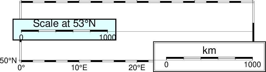
Example of two map scales for a Mercator projection evaluated at 53 degrees north. The left-most scale was placed with -LjML+c53+w1000k+f+l“Scale at 53\232N” while the scale on the right was placed with -LjBR+c53+w1000k+l+f.

Here is the source script for the figure above:

gmt begin GMT_mapscale
	gmt set GMT_THEME cookbook
	gmt basemap -R0/40/50/56 -JM5i -B -LjML+c53+w1000k+f+l"Scale at 53@.N" -F+glightcyan+c0+p
	gmt basemap -LjBR+c53+w1000k+l+f -F+p1p+i+gwhite+c0.1i
	h=$(gmt mapproject -Wh -Di)
	h=$(gmt math -Q $h 2 DIV =)
	lat=$(echo 0 $h | gmt mapproject -I -Di -o1)
	gmt plot -Wfaint -A -N << EOF
>
0	$lat
40	$lat
>
0	50
40	50
EOF
gmt end show

Note that for the purpose of anchor justification (+j) the footprint of the map scale is considered the rectangle that contains the scale and all selected labels and annotations, i.e., the map scale’s bounding box.

3.23.4. Placing directional map roses

Map roses showing the cardinal directions of a map help the reader orient themselves, especially for oblique projections where north-south is not vertically aligned. However, these roses also have ornamental value and can be used on any map projection. As for map scales, a directional map rose is added with basemap or coast and selected by the -Td option. This option accepts the reference point where the map rose’s anchor should be pinned. In addition to the required refpoint and anchor arguments (and their standard modifiers discussed earlier) there is one required and two optional modifiers. The required modifier sets the side:

1. Size of map rose. Use +wsize to specify the full width and height of the rose. A 3 cm rose would require +w3c.

The next two modifiers are optional:

1. Cardinal points. By default only the four cardinal points (W, E, S, N) are included in the rose. You can extend that with the +flevel modifier, where level is 1 [Default], 2, or 3. Selecting 2 will include the two intermediate orientations NW-SE and NE-SW, while 3 adds the four additional orientations WNW-ESE, NNW-SSE, NNE-SSW, and ENE-WSW.

2. Add labels. Do so with +l, which places the current one-letter codes for west, east, south, and north at the four cardinal points. These letters depend on the setting of GMT_LANGUAGE and for the default English we use W, E, S, N, respectively. You can replace these labels with four custom labels via +lw,e,s,n, i.e., four comma-separated labels in the specified order. You can exclude any of the cardinal points from being labeled by giving no label in the corresponding order. E.g., +l”,,Down,Up” would write Down and Up at the south and north cardinal point, respectively. Note that for the plain directional rose only the north annotation will be placed.

Plain and fancy directional map roses. (left) Bare-bones plain rose showing arrow towards north and a cross indicating the cardinal directions, specified by -Tdg0/0+w1i. (middle) Fancy rose obtained by adding +f and +l,,,N to get the north label. (right) Fancy directional rose at level 3 with labels by adding +f3+l.

Here is the source script for the figure above:

gmt begin GMT_dir_rose
	gmt set GMT_THEME cookbook MAP_EMBELLISHMENT_MODE manual
	gmt set FONT_LABEL 10p FONT_TITLE 12p MAP_ANNOT_OBLIQUE lon_horizontal,lat_parallel
	gmt set MAP_TITLE_OFFSET 5p MAP_FRAME_WIDTH 3p FORMAT_GEO_MAP dddF FONT_ANNOT_PRIMARY 10p
	gmt basemap -R-5/5/-5/5 -Jm0.15i -Ba5f -BWSne+gazure1 -Tdg0/0+w1i+jCM -X1i
	gmt basemap -Ba5f -BwSne+gazure1 -Tdg0/0+w1i+f1+jCM+l,,,N -X1.75i
	gmt basemap -R-7/7/-5/5 -Ba5f -BwSnE+gazure1 -Tdg0/0+w1i+f3+l+jCM -X1.75i
gmt end show

3.23.5. Placing magnetic map roses

Map roses showing the magnetic directions of a map are useful when magnetic data are presented, or when declinations are significantly nonzero. However, as for directional roses the magnetic rose also has ornamental value. The magnetic rose consists of two concentric angular scales: The first (outer) ring shows directional angles while the second (inner) ring is optional and portrays the magnetic directions, which differ for nonzero declination. As for style, the two-ring rose looks a bit like a standard compass. As for directional roses, a magnetic map rose is added with basemap or coast and selected by the -Tm option. As for other features, append the required reference point where the magnetic map rose’s anchor should be pinned. There is one required and several optional modifiers. First up is the size:

1. Specify size of map rose. Use +wsize to specify the full width of the rose. A 3 cm rose would imply +w3c.

The remaining modifiers are optional:

1. Specify Declination. To add the inner angular scale, append ddec[/dlabel], where dec is the declination value in decimal or ddd:mm:ss format, and dlabel is an optional string that replaces the default label (which is “d = dec”, with d being a Greek delta and we format the specified declination). Append ddec/- to indicate you do not want any declination label. As an example, consider d11/”Honolulu declination”.

2. Draw the secondary (outer) ring outline. Normally it is not drawn, but you can change that by appending +ppen. For instance, adding +pthin will draw the ring with the selected thin pen.

3. Add labels. As for directional roses you do so with +l, which places the current one-letter codes for west, east, south, and north at the four cardinal points. These letters depend on the setting of GMT_LANGUAGE and for the default English we use W, E, S, N, respectively. You can replace these labels with four custom labels via +lw,e,s,n, i.e., four comma-separated labels in the specified order. You can exclude any of the cardinal points from being labeled by giving no label in the corresponding order. E.g., +l”,,Down,Up” would write Down and Up at the south and north cardinal point, respectively.

4. Draw the primary (inner) ring outline. It is also not normally drawn; change that by appending +ipen. For instance, adding +ithin,blue will draw the ring with the selected thin, blue pen.

5. Set annotation, tick and grid intervals. Each ring has a default annotation [30], tick [5], and grid [1] interval (although here “grid interval” is just a finer tick interval drawn at half tickmark length). Adjust these three intervals with +tintervals. If you selected +d then you must supply two sets of such intervals (i.e., 6 comma-separated values), where the first (primary) set refers to the declination-adjusted ring and the second (secondary) set refers to the directional (outer) ring. If only three intervals are given then we assume you want the same intervals for both rings. As an example, to annotate every 90 degrees and tick every 15 and 5 degrees, add +t90/15/5.

Magnetic direction map rose. This symbol is quite complicated and has many items whose attributes are in part controlled by GMT defaults parameters and in part by the above modifiers. The color-coded legend indicates which parameters controls the font, pen, or color of the correspond item of the rose. This rose was specified by -Tmg-2/0.5+w2.5i+d-14.5+t45/10/5+i0.25p,blue+p0.25p,red+l+jCM. See gmt.conf for more details on the default parameters.

Here is the source script for the figure above:

gmt begin GMT_mag_rose
	gmt set GMT_THEME cookbook MAP_EMBELLISHMENT_MODE manual
	gmt basemap -R-10/-2/12.8812380332/0.661018975345+r -JOc0/0/50/60/7i -B -BWSne -X1.25i --MAP_ANNOT_OBLIQUE=lon_horizontal,lat_parallel --FONT_ANNOT_PRIMARY=12p
	gmt basemap -Tmg-2/0.5+w2.5i+d-14.5+t45/10/5+i0.25p,blue+p0.25p,red+l+jCM \
		--FONT_ANNOT_PRIMARY=9p,Helvetica,blue --FONT_ANNOT_SECONDARY=12p,Helvetica,red --FONT_LABEL=14p,Times-Italic,darkgreen --FONT_TITLE=24p \
		--MAP_TITLE_OFFSET=7p --MAP_FRAME_WIDTH=10p --COLOR_BACKGROUND=green --MAP_DEFAULT_PEN=2p,darkgreen --COLOR_BACKGROUND=darkgreen \
		--MAP_VECTOR_SHAPE=0.5 --MAP_TICK_PEN_SECONDARY=thinner,red --MAP_TICK_PEN_PRIMARY=thinner,blue
	gmt inset begin -DjTR+w2.9i/3.9i+o0.05i -F+p+ggray95
	gmt inset end
	echo "5.5 3.8 GMT DEFAULTS" | gmt text -R0/7/0/4 -Jx1i -F+f14p,Helvetica-Bold+jCM
	gmt text -F+f11.5p+jLM << EOF
4.1 3.50 FONT_TITLE
4.1 3.25 MAP_TITLE_OFFSET
4.1 3.00 MAP_DEGREE_SYMBOL
4.1 2.75 @;blue;FONT_ANNOT_PRIMARY@;;
4.1 2.50 @;blue;MAP_TICK_PEN_PRIMARY@;;
4.1 2.25 @;blue;MAP_ANNOT_OFFSET_PRIMARY@;;
4.1 2.00 @;blue;MAP_TICK_LENGTH_PRIMARY@;;
4.1 1.75 @;red;FONT_ANNOT_SECONDARY@;;
4.1 1.50 @;red;MAP_TICK_PEN_SECONDARY@;;
4.1 1.25 @;red;MAP_ANNOT_OFFSET_SECONDARY@;;
4.1 1.00 @;red;MAP_TICK_LENGTH_SECONDARY@;;
4.1 0.75 @;darkgreen;FONT_LABEL@;;
4.1 0.50 @;darkgreen;MAP_DEFAULT_PEN@;;
4.1 0.25 @;darkgreen;COLOR_BACKGROUND@;;
EOF
gmt end show

3.23.6. Placing color scale bars

Color scale bars are used in conjunction with color-coded surfaces, symbols, lines, or even text, to relate the chosen color to a data value or category. For instance, color images of topography or other gridded data will need a mechanism for users to decode what the colors represent. Typically, we do this by adding a color scale bar on the outside (or inside) of the map boundaries. The module colorbar places the color scale bar, with location and size determined by the -D attributes. As for other map features we must specify the reference and anchor points and any adjustments to them, then supply suitable required and optional modifiers:

1. Give dimensions of color bar. Use +wlength/width to specify the full width and height of the bar. For instance, a 10 cm long bar of height 0.5 cm would imply +w10c/0.5c.

2. Set orientation of color bar. By default, we place a vertically aligned bar. Select a horizontal bar by adding +h.

3. Specify color bar label alignment. By default we place the chosen annotations, scale (i.e., x-axis) label and unit (i.e., y-axis) label on the opposite side of the color scale bar anchor point. Change this with +m and append any combination of a, l, or u to flip the annotations or labels to the opposite side. Append c to plot vertical labels as column text (this cannot be used with +h, obviously).

4. Extend the color bar. You can use the +e modifier to add sidebar triangles for displaying the current back- and foreground colors. Append b (background) or f (foreground) to get the implied side only [Default is both]. Optionally, append triangle height [Default is half the bar width].

5. Add missing data key. Append +n to draw a rectangle with the current NaN color and label it NaN. Optionally, append a replacement text. One example might be +n“No data”.

Color bar placed beneath a map (here truncated). We extended the bar to show background and foreground colors, and used the frame-annotation machinery to add labels. The bar was placed with -DJBC+e.

Here is the source script for the figure above:

gmt begin GMT_colorbar
	gmt set GMT_THEME cookbook
	gmt makecpt -T-15/15 -Cpolar
	gmt basemap -R0/20/0/1 -JM5i -BWse -B
	gmt colorbar -C -Bx+u"@." -By+l@~D@~T -DJBC+e
gmt end show

3.23.7. Placing map legends

Adding map legends is the standard way to communicate what various symbols placed on your map represent. For instance, you may use this mechanism to convey the information that circles are earthquake locations, triangles are places where you ate Thai food, and dashed lines indicate some sort of gang-land demarkation line that you should not cross without paying the locals due respect. Map legends are placed by the module legend, with location and size determined by the various -D attributes. We must again specify the reference and anchor points and any adjustments to them first, then supply suitable required and optional modifiers:

1. Give legend dimensions. You must specify the required legend width, while legend height is optional and if not given is computed based on the contents of the legend. The syntax is therefore +wwidth[/height] in your desired plot units. Thus, +w12c sets the legend width as 12 cm but the height will become whatever is needed to contain the information.

2. Set line-spacing. You may optionally specify the line-spacing used for the setting of the legend. The legend will typically consist of several lines that may or may not contain text, but the spacing between these lines are controlled by the chosen line-spacing factor times the current primary annotation font setting, i.e., FONT_ANNOT_PRIMARY. The default line spacing factor is 1.1; change this with +llinefactor.

Example of a map legend placed with legend. Apart from the placement and dimensions discussed here, legend reads macro commands that specifies each item of the legend, including colors, widths of columns, the number of columns, and presents a broad selection of items. Here, we simply used -Dx0/0+w14c+jBL.

Here is the source script for the figure above:

gmt begin GMT_legend
gmt set GMT_THEME cookbook
cat <<EOF > table.txt
H 24 Times-Roman Eight Largest Cities in North America
D 1p
N 6 22 16 20 20 8 8
V 0.25p
S 0.15i c 0.1i snow1 -
L - - C City Name
L - - C Country
L - - C Population
L - - C Climate
L - - C WC?
L - - C OL?
D 0 1p
F lightgreen
S 0.15i c 0.1i red 0.25p
L - - R Mexico City
L - - R Mexico
L - - R 8,851,080
L - - R Tropical
L - - C Y
L - - C Y
F -
S 0.15i c 0.1i orange 0.25p
L - - R New York City
L - - R USA
L - - R 8,405,837
L - - R Tempered
L - - C Y
L - - C N
S 0.15i c 0.1i yellow 0.25p
L - - R Los Angeles
L - - R USA
L - - R 3,904,657
L - - R Subtropical
L - - C Y
L - - C Y
F lightblue
S 0.15i c 0.1i green 0.25p
L - - R Toronto
L - - R Canada
L - - R 2,795,060
L - - R Tempered
L - - C N
L - - C N
F -
S 0.15i c 0.1i blue 0.25p
L - - R Chicago
L - - R USA
L - - R 2,714,856
L - - R Tempered
L - - C Y
L - - C N
S 0.15i c 0.1i cyan 0.25p
L - - R Houston
L - - R USA
L - - R 2,714,856
L - - R subtropical
L - - C N
L - - C N
F lightred
S 0.15i c 0.1i magenta 0.25p
L - - R Havana
L - - R Cuba
L - - R 2,106,146
L - - R Tropical
L - - C N
L - - C N
F lightblue
S 0.15i c 0.1i white 0.25p
L - - R Montreal
L - - R Canada
L - - R 1,649,519
L - - R Tempered
L - - C N
L - - C Y
D 1p
V 1p
F -
N 1
L 9 4 R Information from Wikipedia
G 0.05i
T Many of these cities have hosted World Cup Soccer (WC) and some
T have hosted the Olympics (OL).  The rest is just some basic information
T about each city, such as climate and population.  Of course, this is all
T an excuse to demonstrate variable-width tables and row coloring.
G 0.15i
EOF
cat << EOF > t.cpt
1	red
2	orange
3	yellow
4	green
5	blue
6	cyan
7	magenta
8	white
EOF
gmt legend -Dx0/0+w5.6i+jBL+l1.2 -C0.05i -F+p+gsnow1 -B0 table.txt --FONT_LABEL=12p
rm -f table.txt t.cpt
gmt end show

3.23.8. Placing raster and EPS images on maps

When preparing posters for meetings one will often need to include the organization’s logo, which may be available to you as an Encapsulated PostScript File (EPS) or as a raster image, such as PNG or JPG. At other times, you may wish to place photos or other raster images on your map. The module image can help with this, and like the other map feature placements it requires a reference point and its optional adjustments via the -D option. In addition, we require one (of two) modifiers to determine the image size.

1. Specify image width. This is a required modifier and is set via +wwidth[/height]. If height is specified as 0 then we compute the height from width and the aspect ratio of the image, for instance +w4c/0. If width is negative the we use its absolute value as width but interpolate the image in PostScript to the device resolution.

2. Specify image resolution. For raster images (not EPS) you may instead specify the size of the plotted image by specifying its resolution in dots per inch, via +rdpi. The actual size of the images is then controlled by its number of pixels times the dpi.

3. Enable image replication. For raster images (not EPS) you may optionally append +nnx[/ny] to indicate that you want the source image to be replicated that many times in the two directions, resulting in a tiling of the map using the selected image. This may be useful in conjunction with an active clip path set by clip.

Placement of EPS and raster images. (left) The US National Science Foundation (NSF) has generously funded the development of GMT and their JPG logo is reproduced here via -DjML+w1.5i+o0.1i. (right) The School of Ocean and Earth Science and Technology at the University of Hawaii at Manoa hosts the gmt server and its EPS logo is shown via -DjMR+o0.1i+w2i.

Here is the source script for the figure above:

gmt begin GMT_images
	gmt set GMT_THEME cookbook
	gmt image @nsf1.jpg -R0/2/0/1 -JX5i/1.6i -B0 -DjML+w1.5i+o0.1i/0i
	gmt image @soest.eps -DjMR+o0.1i/0i+w2i
gmt end show

3.23.9. Placing a GMT logo on maps

It is possible to overlay the GMT logo on maps as well, using the module gmtlogo. Like other features it requires reference and anchor points and their optional adjustments via the -D option. In addition, we require one modifier to set the logo’s size.

1. Specify logo width. This is a required modifier and is set via +wwidth. The height is automatically set (it is half the width). To place a 5 cm wide GMT logo, append +w5c.

Placement of the GMT logo. The logo itself only has a size modifier but the gmtlogo module allows additional attributes such as a background map panel.

Here is the source script for the figure above:

gmt logo -Dx0/0+w5.458i -X0 -Y0 --GMT_THEME=cookbook -view GMT_coverlogo

3.23.10. Placing map insets

Our penultimate map embellishment is the map inset. A map inset may appear to be the easiest feature to add since it only consists of an empty map panel. What you put in this panel is up to you (and we will show some examples). However, unlike the other map features there are two ways to specify the placement of the map inset. The first is the standard way of specifying the reference and anchor points and the inset dimensions, while the second specifies a subregion in the current plot that should be designated the map inset area. Depending on the map projection this may or may not be a rectangular area. Map insets are produced by the module inset and located via the -D option. Unless you use the reference point approach you must first append xmin/xmax/ymin/ymax[+r][+uunit], where the optional unit modifier +u indicates that the four coordinates to follow are projected distances (e.g., km, miles). If the unit modifier is missing then we assume the coordinates are map coordinates (e.g., geographic west, east, south, and north). For oblique projections you may wish to specify the domain using the lower-left and upper-right coordinates instead (similar to how the -R option works), by adding +r. Some optional modifiers are available:

1. Set inset size. If you specified a reference point then you must also specify the inset dimensions with the +wwidth[/height], where height defaults to width if not given. Append the unit of the dimensions, which may be distance units such as km, feet, etc., and the map projection will be used to determine inset dimensions on the map. For instance, +w300k/200k is a 300x200 km region (which depends on the projection) while +w5c is a 5cm square box.

2. Save the location and dimensions. For all but the simplest of map insets you will need to know the exact location of the resulting inset and its dimensions. For instance, if you specified the inset using the TR anchor point and a width and height of 100 km you will need to know what this means in terms of positions on the map in plot units. In terms of the modifiers this would be jTR+w100k. See the figure caption for an example.

Demonstration of how a map inset may be used to place a global overview map as an inset in a regional map. Main map shows the regional area of Australia. We place an inset in the upper right area with -DjTR+w3.8c+o0.4c/0.25c. See Example (44) Map insets for more details.

Here is the source script for the figure above:

gmt begin GMT_inset
	gmt set GMT_THEME cookbook
	gmt coast -R110E/170E/44S/9S -JM6i -B -BWSne -Wfaint -N2/1p  -EAU+gbisque -Gbrown -Sazure1 -Da -Xc --FORMAT_GEO_MAP=dddF
	gmt inset begin -DjTR+w1.5i+o0.15i -F+gwhite+p1p+s -C0.05i
	gmt coast -Rg -JG120/30S/ -Da -Gbrown -A5000 -Bg -Wfaint -EAU+gbisque
	gmt inset end
gmt end show

3.23.11. Placing a vertical scale on maps

Our final embellishment is reserved for wiggles plotted along track with wiggle and is activated as an option within that module. Like other features, it requires reference and anchor points and their optional adjustments via the -D option. In addition, we offer a few modifier to set the scale bar’s remaining attributes:

1. Specify vertical scale bar length. This is a required modifier and is set via +llength. The length is given in the data (z) units of your plot. To indicate that your vertical scale bar should reflect 100 nTesla, append +l100. The actual dimension of the scale bar on your map depends on the data scale set in wiggle via -Z.

2. Place the label on the left side of the vertical scale bar. This is an optional modifier and is set via +m. By default, the scale bar has open teeth pointing right and a label on that side. The m moves the label to the left and reverses the teeth direction as well.

3. Add a unit to the vertical scale bar label. This is an optional modifier and is set via +uunit. To append nT (nTesla) to the label you would specify +unT.

Placement of a vertical scale bar. As for other embellishments the wiggle module allows additional attributes such as a background map panel.

Here is the source script for the figure above:

gmt begin GMT_vertscale
	gmt set GMT_THEME cookbook
	gmt math -T-8/6/0.01 -N3/0 -C2 T 3 DIV 2 POW NEG EXP T PI 2 MUL MUL COS MUL 50 MUL = t.txt
	gmt wiggle -R-10/10/-3/3 -JM6i -B -Z100i -DjRM+w100+lnT t.txt -Tfaint -W1p -BWSne --MAP_FRAME_TYPE=plain
gmt end show

3.24. Grid file format specifications

GMT has the ability to read and write grids using more than one grid file format (see Table grdformats for supported format and their IDs). For reading, GMT will automatically determine the format of grid files, while for writing you will normally have to append =ID to the filename if you want GMT to use a different format than the default. The automatic reading procedure follows an heuristic where certain formats are tentatively decoded with GMT internal drivers and if they fail than we resort to use the GDAL library to do the readings. This normally works pretty well but in case of failure (e.g. a GMT driver failed to read binary file with a separate header that also could have been stored in an ASCII file with embed header) the user should explicitly try to force a reading via GDAL. That is, to append a =gd suffix to file name.

By default, GMT will create new grid files using the nf format; however, this behavior can be overridden by setting the IO_GRIDFILE_FORMAT defaults parameter to any of the other recognized values (or by appending =ID).

GMT can also read netCDF grid files produced by other software packages, provided the grid files satisfy the COARDS and Hadley Centre conventions for netCDF grids. Thus, products created under those conventions (provided the grid is 2-, 3-, 4-, or 5-dimensional) can be read directly by GMT and the netCDF grids written by GMT can be read by other programs that conform to those conventions. Three such programs are ncview, Panoply, and ncBrowse ; others can be found on the netCDF website. Note that although many additional programs can read netCDF files, some are unable to read netCDF 4 files (if data compression has been applied).

In addition, users with some C-programming experience may add their own read/write functions and link them with the GMT library to extend the number of predefined formats. Technical information on this topic can be found in the source file gmt_customio.c. Users who are considering this approach should contact the GMT team for guidance.

ID	Explanation
	GMT 4 netCDF standard formats
nb	GMT netCDF format (8-bit integer, COARDS, CF-1.5)
ns	GMT netCDF format (16-bit integer, COARDS, CF-1.5)
ni	GMT netCDF format (32-bit integer, COARDS, CF-1.5)
nf	GMT netCDF format (32-bit float, COARDS, CF-1.5)
nd	GMT netCDF format (64-bit float, COARDS, CF-1.5)
	GMT 3 netCDF legacy formats
cb	GMT netCDF format (8-bit integer, depreciated)
cs	GMT netCDF format (16-bit integer, depreciated)
ci	GMT netCDF format (32-bit integer, depreciated)
cf	GMT netCDF format (32-bit float, depreciated)
cd	GMT netCDF format (64-bit float, depreciated)
	GMT native binary formats
bm	GMT native, C-binary format (bit-mask)
bb	GMT native, C-binary format (8-bit integer)
bs	GMT native, C-binary format (16-bit integer)
bi	GMT native, C-binary format (32-bit integer)
bf	GMT native, C-binary format (32-bit float)
bd	GMT native, C-binary format (64-bit float)
	Miscellaneous grid formats
rb	SUN raster file format (8-bit standard)
rf	GEODAS grid format GRD98 (NCEI)
sf	Golden Software Surfer format 6 (32-bit float)
sd	Golden Software Surfer format 7 (64-bit float)
af	Atlantic Geoscience Center AGC (32-bit float)
ei	ESRI Arc/Info ASCII Grid Interchange format (ASCII integer)
ef	ESRI Arc/Info ASCII Grid Interchange format (ASCII float)
gd	Import/export via GDAL

Because some formats have limitations on the range of values they can store it is sometimes necessary to provide more than simply the name of the file and its ID on the command line. For instance, a native short integer file may use a unique value to signify an empty node or NaN, and the data may need translation and scaling prior to use. Therefore, all GMT programs that read or write grid files will decode the given filename as follows:

name[=ID][+ddivisor][+ninvalid][+ooffset][+sscale]

where anything in brackets is optional. If you are reading a grid then no ID is needed: just continue to pass the name of the grid file. However, if you write another format than the default netCDF you must append the =ID string, where ID is the format code listed above. In addition, should you want to (1) multiply the data by a scale factor (or alternatively divide the data by a divisor), and (2) add a constant offset you must append the +sscale (or +ddivisor) and +ooffset modifiers. Finally, if you need to indicate that a certain data value should be interpreted as a NaN (not-a-number) you must append +ninvalid modifier to file name. For output, you may specify scale as a for auto-adjusting the scale and/or offset of packed integer grids (=ID+sa is a shorthand for =ID+sa+oa).

Note: Users are allowed to name their grid files anything they want. However, if you tend to use what could look like modifier-sequences to GMT (e.g., using filenames like data.grid+o4) you can prevent any confusion by using either the GMT-recommended “.grd” or “.nc” as grid file extensions (e.g., data.my+o4.grd). Since valid modifiers are appended to a file name, finding such an extension simplifies parsing.

Note that the GMT netCDF and native binary grids store the grid scale and offset in the file, hence if you specify these attributes when writing a file then upon reading the grid these settings will automatically take effect. You can override them by supplying different scales and offsets, of course. For the grid formats that do not store these attributes you will need to supply them both when reading and writing.

Some of the grid formats allow writing to standard output and reading from standard input which means you can connect GMT programs that operate on grid files with pipes, thereby speeding up execution and eliminating the need for large, intermediate grid files. You specify standard input/output by leaving out the filename entirely. That means the “filename” will begin with “=ID”. Note that the netCDF format does not allow piping.

Everything looks clearer after a few examples:

• To write a native binary float grid file, specify the name as my_file.f4=bf .

• To read a native short integer grid file, multiply the data by 10 and then add 32000, but first let values that equal 32767 be set to NaN, use the filename my_file.i2=bs+s10+o32000+n32767.

• To read a Golden Software “surfer” format 6 grid file, just pass the file name, e.g., my_surferfile.grd.

• To read a 8-bit standard Sun raster file (with values in the 0–255 range) and convert it to a 1 range, give the name as rasterfile+s7.84313725e-3+o-1 (i.e., 1/127.5).

• To write a native binary short integer grid file to standard output after subtracting 32000 and dividing its values by 10, give filename as =bs+s0.1+o-3200.

• To write an 8-bit integer netCDF grid file with an auto-adjusted offset, give filename as =nb+oa.

• To read a short integer .bil grid file stored in binary and and force the reading via GDAL, add suffix =gd as in n45_e008_1arc_v3.bil=gd

• To write a lossless, deflate compressed, and tiled GeoTIFF grid (or image) use, output.tif=gd:GTiff+cTILED=YES+cCOMPRESS=DEFLATE+cPREDICTOR=3 See also Writing grids and images as well as available options for each output format from the GDAL driver documentation, for example

Programs that both read and/or write more than one grid file may specify different formats and/or scaling for the files involved. The only restriction with the embedded grid specification mechanism is that no grid files may actually use the “=” character as part of their name (presumably, a small sacrifice).

One can also define special file suffixes to imply a specific file format; this approach represents a more intuitive and user-friendly way to specify the various file formats. The user may create a file called gmt.io in the current directory or home directory, or in the directory ~/.gmt and define any number of custom formats. The following is an example of a gmt.io file:

# GMT i/o shorthand file # It can have any number of comment lines like this one anywhere # suffix format_id scale offset NaN Comments
grd	nf	-	-	-	Default format
b	bf	-	-	-	Native binary floats
i2	bs	-	-	32767	2-byte integers with NaN value
ras	rb	-	-	-	Sun raster files
byte	bb	-	-	255	Native binary 1-byte grids
bit	bm	-	-	-	Native binary 0 or 1 grids
mask	bm	-	-	0	Native binary 1 or NaN masks
faa	bs	0.1	-	32767	Native binary gravity in 0.1 mGal
ns	ns	a	a	-	16-bit integer netCDF grid with auto-scale and auto-offset

These suffices can be anything that makes sense to the user. To activate this mechanism, set parameter IO_GRIDFILE_SHORTHAND to TRUE in your gmt.conf file. Then, using the filename stuff.i2 is equivalent to saying stuff.i2=bs+n32767, and the filename wet.mask means wet.mask=bm+n0. For a file intended for masking, i.e., the nodes are either 1 or NaN, the bit or mask format file may be as small as 1/32 the size of the corresponding grid float format file.

3.25. Modifiers for changing units of grid coordinates

A few GMT tools require that the two horizontal dimensions be specified in meters. One example is grdfft which must compute the 2-D Fourier transform of a grid and evaluate wave numbers in the proper units (1/meter). There are two situations where the user may need to change the coordinates of the grid passed to such programs:

• You have a geographic grid (i.e., in longitude and latitude). Simply supply the -fg option and your grid coordinates will automatically be converted to meters via a “Flat Earth” approximation on the currently selected ellipsoid (Note: This is only possible in those few programs that require this capability. In general, -fg is used to specify table coordinates).

• You have a Cartesian grid but the units are not meters (e.g., they may perhaps be in km or miles). In this case you may append the file modifier +uunit, where unit is one of non-angular units listed in Table distunits. For example, reading in the grid (which has distance units of km) and converting distances to meters is done by specifying the filename as filename+uk. On output, any derived grids will revert to their original units unless you specify another unit modifier to the output grid. This may be used, for instance, to save the original grid with distances in meters using some other unit.

For convenience, we also support the inverse translation, i.e., +Uunit. This modifier can be used to convert your grid coordinates from meters to the specified unit. Example (28) Mixing UTM and geographic data sets shows a case where this is being used to change an UTM grid in meters to km. These modifiers are only allowed when map projections are not selected (or are Cartesian).

3.26. Modifiers for COARDS-compliant netCDF files

When the netCDF grid file contains more than one 2-dimensional variable, GMT programs will load the first such variable in the file and ignore all others. Alternatively, the user can select the required variable by adding the suffix “?varname” to the grid file name. For example, to get information on the variable “slp” in file , use:

gmt grdinfo "file.nc?slp"

Since COARDS-compliant netCDF files are the default, the additional suffix “=nf” can be omitted.

If there are no 2-dimensional variables and no specific variable was selected, we default to the first higher-dimensional matrix and select the first layer.

In case the named grid is 3-dimensional, GMT will load the first (bottom) layer. If another layer is required, either add “[index]” or “(level)”, where index is the index of the third (depth) variable (starting at 0 for the first layer) and level is the numerical value of the third (depth) variable associated with the requested layer. To indicate the second layer of the 3-D variable “slp” use as file name: file.nc?slp[1].

When you supply the numerical value for the third variable using “(level)”, GMT will pick the layer closest to that value. No interpolation is performed (for such interpolations, see grdinterpolate).

Note that the question mark, brackets and parentheses have special meanings on Unix-based platforms. Therefore, you will need to either escape these characters, by placing a backslash in front of them, or place the whole file name plus modifiers between single quotes or double quotes.

A similar approach is followed for loading 4-dimensional grids. Consider a 4-dimensional grid with the following variables:

lat(lat): 0, 1, 2, 3, 4, 5, 6, 7, 8, 9
lon(lon): 0, 1, 2, 3, 4, 5, 6, 7, 8, 9
depth(depth): 0, 10, 20, 30, 40, 50, 60, 70, 80, 90
time(time): 0, 12, 24, 36, 48
pressure(time,depth,lat,lon): (5000 values)

To get information on the 10x10 grid of pressure at depth 10 and at time 24, one would use:

gmt grdinfo "file.nc?pressure[2,1]"

or (only in case the coordinates increase linearly):

gmt grdinfo "file.nc?pressure(24,10)"

Programs that generally deal with columns of one-dimensional data, like or can use multi-dimensional netCDF files in a very similar way. If a variable in a netCDF file is one-dimensional, there is nothing more needed than name the variables on the command line. For example:

gmt plot "file.nc?lon/lat" ...
gmt convert "file.nc?time/lat/lon"

If one or more of the selected variables are two-dimensional, and have the same leading dimension as the other selected variables they will be plotted in their entirety. For example, if a netCDF files contains 6 time steps recording temperature at 4 points, and the variable temp is a 6 by 4 array, then the command gmt convert "file.nc?time/temp" can result in:

2012-06-25T00:00:00 20.1 20.2 20.1 20.3
2012-06-25T12:00:00 24.2 23.2 24.5 23.5
2012-06-26T00:00:00 16.1 16.2 16.1 16.3
2012-06-26T12:00:00 22.1 23.0 23.9 23.5
2012-06-27T00:00:00 17.5 16.9 17.2 16.8
2012-06-27T12:00:00 27.2 27.2 27.5 27.5

If, for example, only the second temperature column is needed, use gmt convert "file.nc?time/temp[1]" (indices start counting at 0).

The COARDS conventions set restrictions on the names that can be used for the units of the variables and coordinates. For example, the units of longitude and latitude are “degrees_east” and “degrees_north”, respectively. Here is an example of the header of a COARDS compliant netCDF file (to be obtained using ncdump):

netcdf M2_fes2004 {
dimensions:
        lon = 2881 ;
        lat = 1441 ;
variables:
        float lon(lon) ;
                lon:long_name = "longitude" ;
                lon:units = "degrees_east" ;
                lon:actual_range = 0., 360. ;
        float lat(lat) ;
                lat:long_name = "latitude" ;
                lat:units = "degrees_north" ;
                lat:actual_range = -90., 90. ;
        short amp(lat, lon) ;
                amp:long_name = "amplitude" ;
                amp:unit = "m" ;
                amp:scale_factor = 0.0001 ;
                amp:add_offset = 3. ;
                amp:_FillValue = -32768s ;
        short pha(lat, lon) ;
                pha:long_name = "phase" ;
                pha:unit = "degrees" ;
                pha:scale_factor = 0.01 ;
                pha:_FillValue = -32768s ;

This file contains two grids, which can be plotted separately using the names M2_fes2004.nc?amp and M2_fes2004.nc?pha. The attributes long_name and unit for each variable are combined in GMT to a single unit string. For example, after reading the grid y_unit equals latitude [degrees_north]. The same method can be used in reverse to set the proper variable names and units when writing a grid. However, when the coordinates are set properly as geographical or time axes, GMT will take care of this. The user is, however, still responsible for setting the variable name and unit of the z-coordinate. The default is simply “z”.

3.27. Modifiers to read and write grids and images via GDAL

GMT can read and write a variety of grid and image formats via GDAL. This extends the capability of GMT to handle data sets from a variety of sources.

3.27.1. Reading multi-band images

grdimage and image both lets the user select individual bands in a multi-band image file and treats the result as an image (that is the values, in the 0–255 range, are treated as colors, not data). To select individual bands you use the +bband-number mechanism that must be appended to the image filename. Here, band-number can be the number of one individual band (the counting starts at zero), or it could be a comma-separated list of bands. For example

gmt image jpeg_image_with_three_bands.jpg+b0 -jpg gray

will plot only the first band (i.e., the red band) of the jpeg image as a gray-scale image, and

gmt image jpeg_image_with_three_bands.jpg+b2,1,0 -jpg bgr

will plot the same image in color but where the RGB band order has been reversed.

Instead of treating them as images, all other GMT programs that process grids can read individual bands from an image but will consider the values to be regular data. For example, let multiband be the name of a multi-band file with a near infrared component in band 4 and red in band 3. We will compute the NDVI (Normalized Difference Vegetation Index), which is defined as NDVI = (NIR - R) / (NIR + R), as

gmt grdmath multiband=gd+b3 multiband=gd+b2 SUB multiband=gd+b3 \
            multiband=gd+b2 ADD DIV = ndvi.nc

The resulting grid ndvi.nc can then be plotted as usual.

3.27.2. Reading more complex multi-band IMAGES or GRIDS

It is also possible to access to sub-datasets in a multi-band grid. The next example shows how we can extract the SST from the MODIS file A20030012003365.L3m_YR_NSST_9 that is stored in the HDF “format”. We need to run the GDAL program gdalinfo on the file because we first must extract the necessary metadata from the file:

gdalinfo A20030012003365.L3m_YR_NSST_9
Driver: HDF4/Hierarchical Data Format Release 4
Files: A20030012003365.L3m_YR_NSST_9
Size is 512, 512
Coordinate System is `'
Metadata:
 Product Name=A20030012003365.L3m_YR_NSST_9
 Sensor Name=MODISA
 Sensor=
 Title=MODISA Level-3 Standard Mapped Image
...
 Scaling=linear
 Scaling Equation=(Slope*l3m_data) + Intercept = Parameter value
 Slope=0.000717185
 Intercept=-2
 Scaled Data Minimum=-2
 Scaled Data Maximum=45
 Data Minimum=-1.999999
 Data Maximum=34.76
Subdatasets:
 SUBDATASET_1_NAME=HDF4_SDS:UNKNOWN:"A20030012003365.L3m_YR_NSST_9":0
 SUBDATASET_1_DESC=[2160x4320] l3m_data (16-bit unsigned integer)
 SUBDATASET_2_NAME=HDF4_SDS:UNKNOWN:"A20030012003365.L3m_YR_NSST_9":1
 SUBDATASET_2_DESC=[2160x4320] l3m_qual (8-bit unsigned integer)

Now, to access this file with GMT we need to use the =gd mechanism and append the name of the sub-dataset that we want to extract. Here, a simple example using grdinfo would be

gmt grdinfo A20030012003365.L3m_YR_NSST_9=gd?HDF4_SDS:UNKNOWN:"A20030012003365.L3m_YR_NSST_9":0

HDF4_SDS:UNKNOWN:A20030012003365.L3m_YR_NSST_9:0: Title: Grid imported via GDAL
HDF4_SDS:UNKNOWN:A20030012003365.L3m_YR_NSST_9:0: Command:
HDF4_SDS:UNKNOWN:A20030012003365.L3m_YR_NSST_9:0: Remark:
HDF4_SDS:UNKNOWN:A20030012003365.L3m_YR_NSST_9:0: Gridline node registration used
HDF4_SDS:UNKNOWN:A20030012003365.L3m_YR_NSST_9:0: Grid file format: gd = Import through GDAL (convert to float)
HDF4_SDS:UNKNOWN:A20030012003365.L3m_YR_NSST_9:0: x_min: 0.5 x_max: 4319.5 x_inc: 1 name: x nx: 4320
HDF4_SDS:UNKNOWN:A20030012003365.L3m_YR_NSST_9:0: y_min: 0.5 y_max: 2159.5 y_inc: 1 name: y ny: 2160
HDF4_SDS:UNKNOWN:A20030012003365.L3m_YR_NSST_9:0: z_min: 0 z_max: 65535 name: z
HDF4_SDS:UNKNOWN:A20030012003365.L3m_YR_NSST_9:0: scale_factor: 1 add_offset: 0

Be warned, however, that things are not yet completed because while the data are scaled according to the equation printed above (“Scaling Equation=(Slope*l3m_data) + Intercept = Parameter value”), this scaling is not applied by GDAL on reading so it cannot be done automatically by GMT. One solution is to do the reading and scaling via grdmath first, i.e.,

gmt grdmath A20030012003365.L3m_YR_NSST_9=gd?HDF4_SDS:UNKNOWN:"A20030012003365.L3m_YR_NSST_9":0 \
            0.000717185 MUL -2 ADD = sst.nc

then plot the sst.nc directly.

3.27.3. Writing grids and images

Saving images in the common raster formats is possible but, for the time being, only from grdimage and even that is restricted to raster type information. That is, vector data (for instance, coast lines) or text will not be saved. To save an image with grdimage use the -Aoutimg=driver mechanism, where driver is the driver code name used by GDAL (e.g. GTiff) (run gdal_translate --formats for the full list.)

For all other programs that create grids, it is also possible to save them using GDAL. To do it one need to use the =gd appended with the necessary information regarding the driver and the data type to use. Generically, =gd[+sscale][+ooffset][+nnan][:<driver>[/dataType][+coptions]] where driver is the same as explained above and dataType is a 2 or 3 chars code from: u8|u16|i16|u32|i32|float32, and where i|u denotes signed|unsigned. If not provided the default type is float32. Both driver names and data types are case insensitive. The options is a list of one or more concatenated number of GDAL -co options. For example, to write a lossless JPG2000 grid one would append +cQUALITY=100+cREVERSIBLE=YES+cYCBCR420=NO Note: You will have to specify a nan value for integer data types unless you wish that all NaN data values should be replaced by zero.

Consider setting IO_NC4_DEFLATION_LEVEL to reduce file size and to further increase read/write performance. Especially when working with subsets of global grids, masks, and grids with repeating grid values, the improvement is usually significant.

3.28. The NaN data value

For a variety of data processing and plotting tasks there is a need to acknowledge that a data point is missing or unassigned. In the “old days”, such information was passed by letting a value like -9999.99 take on the special meaning of “this is not really a value, it is missing”. The problem with this scheme is that -9999.99 (or any other floating point value) may be a perfectly reasonable data value and in such a scenario would be skipped. The solution adopted in GMT is to use the IEEE concept Not-a-Number (NaN) for this purpose. Mathematically, a NaN is what you get if you do an undefined mathematical operation like 0/0; in ASCII data files they appear as the textstring NaN. This value is internally stored with a particular bit pattern defined by IEEE so that special action can be taken when it is encountered by programs. In particular, a standard library function called isnan is used to test if a floating point is a NaN. GMT uses these tests extensively to determine if a value is suitable for plotting or processing (if a NaN is used in a calculation the result would become NaN as well). Data points whose values equal NaN are not normally plotted (or plotted with the special NaN color given in gmt.conf). Several tools such as xyz2grd, gmtmath, and grdmath can convert user data to NaN and vice versa, thus facilitating arbitrary masking and clipping of data sets. Note that a few computers do not have native IEEE hardware support. At this point, this applies to some of the older Cray super-computers. Users on such machines may have to adopt the old ‘-9999.99’ scheme to achieve the desired results.

Data records that contain NaN values for the x or y columns (or the z column for cases when 3-D Cartesian data are expected) are usually skipped during reading. However, the presence of these bad records can be interpreted in two different ways, and this behavior is controlled by the IO_NAN_RECORDS defaults parameter. The default setting (gap) considers such records to indicate a gap in an otherwise continuous series of points (e.g., a line), and programs can act upon this information, e.g., not to draw a line across the gap or to break the line into separate segments. The alternative setting (bad) makes no such interpretation and simply reports back how many bad records were skipped during reading; see Section Data gap detection: The -g option for details.

3.29. Directory parameters

GMT versions prior to GMT 5 relied solely on several environment variables ($GMT_SHAREDIR, $GMT_DATADIR, $GMT_USERDIR, and $GMT_TMPDIR), pointing to folders with data files and program settings. Beginning with version 5, some of these locations are now (also or exclusively) configurable with the gmtset utility. When an environment variable has an equivalent parameter in the gmt.conf file, then the parameter setting will take precedence over the environment variable.

Variable $GMT_SHAREDIR

was sometimes required in previous GMT versions to locate the GMT share directory where all run-time support files such as coastlines, custom symbols, PostScript macros, color tables, and much more reside. If this parameter is not set (default), GMT will make a reasonable guess of the location of its share folder. Setting this variable is usually not required and recommended only under special circumstances.

Variable $GMT_DATADIR and parameter DIR_DATA

may point to one or more directories where large and/or widely used data files can be placed. All GMT programs look in these directories when a file is specified on the command line and it is not present in the current directory. This allows maintainers to consolidate large data files and to simplify scripting that use these files since the absolute path need not be specified. Separate multiple directories with commas. Any directory name that ends in a trailing slash (/) will be searched recursively (not under Windows).

Variable $GMT_USERDIR

may point to a directory where the user places custom configuration files (e.g., an alternate coastline.conf file, preferred default settings in gmt.conf, custom symbols and color palettes, math macros for gmtmath and grdmath, and shorthands for gridfile extensions via gmt.io). When $GMT_USERDIR is not defined, then the default value $HOME/.gmt will be assumed. Users may also place their own data files in this directory as GMT programs will search for files given on the command line in both DIR_DATA and $GMT_USERDIR.

Variable $GMT_CACHEDIR

may point to a directory where the user places cached data files downloaded from the GMT data server. When $GMT_CACHEDIR is not defined, then the default value $HOME/.gmt/cache will be assumed. The cache directory can be emptied by running gmt gmt clear cache.

Variable $GMT_TMPDIR

may indicate the location, where GMT will write its state parameters via the two files gmt.history and gmt.conf. If $GMT_TMPDIR is not set, these files are written to GMT session directory [for modern mode] or the current directory [for classic mode].

Parameter DIR_DCW

specifies where to look for the optional Digital Charts of the World database (for country coloring or selections).

Parameter DIR_GSHHG

specifies where to look for the required Global Self-consistent Hierarchical High-resolution Geography database.

Note that files whose full path is given will never be searched for in any of these directories.

3.30. Footnotes

[7]

Vicenty, T. (1975), Direct and inverse solutions of geodesics on the ellipsoid with application of nested equations, Surv. Rev., XXII(176), 88–93.

[8]

PostScript definition. In the typesetting industry a slightly different definition of point (1/72.27 inch) is used, presumably to cause needless trouble.

[9]

Choose between SI and US default units by modifying in the GMT share directory.

[10]

To remain backwards compatible with GMT 4 we will also look for but only if cannot be found.

[16]

To keep PostScript files small, such comments are by default turned off; see PS_COMMENTS to enable them.

[17]

For an overview of color systems such as HSV, see Chapter Color Systems and Artificial Illumination.

[18]

Convert other graphics formats to Sun ras format using GraphicsMagick’s or ImageMagick’s convert program.