4. Standardized command line options
Most of the programs take many of the same arguments such as those related to setting the data region, the map projection, etc. The switches in Table switches have the same meaning in all the programs (although some programs may not use all of them). These options will be described here as well as in the manual pages, as is vital that you understand how to use these options. We will present these options in order of importance (some are used a lot more than others).
Standard option |
Description |
|---|---|
Define tick marks, annotations, and labels for basemaps and axes |
|
Select a map projection or coordinate transformation |
|
Define the extent of the map/plot region |
|
Plot a time-stamp, by default in the lower left corner of page |
|
Select verbose operation; reporting on progress |
|
Set the x-coordinate for the plot origin on the page |
|
Set the y-coordinate for the plot origin on the page |
|
Associate aspatial data from OGR/GMT files with data columns |
|
Select binary input and/or output |
|
Advance plot focus to selected (or next) subplot panel |
|
Replace user nodata values with IEEE NaNs |
|
Only process data records that match a pattern |
|
Specify the data content on a per column basis |
|
Identify data gaps based on supplied criteria |
|
Specify that input/output tables have header record(s) |
|
Specify which input columns to read |
|
Specify how spherical distances should be computed |
|
Add a legend entry for the symbol or line being plotted |
|
Specify grid interpolation settings |
|
Specify which output columns to write |
|
Control perspective views for plots |
|
Specify which input rows to read or output rows to write |
|
Set grid registration [Default is gridline] |
|
Control output of records containing one or more NaNs |
|
Change layer transparency |
|
Convert selected coordinate to repeating cycles |
|
Set number of cores to be used in multi-threaded applications |
|
Assume input geographic data are (lat,lon) and not (lon,lat) |
4.1. Data domain or map region: The -R option
Syntax
- -Rxmin/xmax/ymin/ymax[+r][+uunit]
Specify the region of interest.
Description
The -R option defines the map region or data domain of interest. It may be specified in one of several ways (options 1 and 3 are shown in panels a) and b) respectively of the Figure Map region):
-Rxmin/xmax/ymin/ymax. This is the standard way to specify Cartesian data domains and geographic regions when using map projections where meridians and parallels are rectilinear, where xmin, xmax, ymin, and ymax refer to the data limits.
-Rxmin/xmax/ymin/ymax+uunit. Append +uunit to the option 1 to specify a region in projected units (e.g., UTM meters) where xmin/xmax/ymin/ymax are Cartesian projected coordinates compatible with the chosen projection and unit is an allowable distance unit [e]. The coordinates are relative to the standard longitude and latitude indicated in the projection (-J). For projected regions centered on (0,0) you may use the short-hand -Rhalfwidth[/halfheight]+uunit, where halfheight defaults to halfwidth if not given. This short-hand requires the +u modifier.
-Rxlleft/ylleft/xuright/yuright+r. This form is useful for map projections that are oblique, making meridians and parallels poor choices for map boundaries. Here, we instead specify the lower left corner and upper right corner geographic coordinates, followed by the modifier +r. This form guarantees a rectangular map even though lines of equal longitude and latitude are not straight lines.
-Rg or -Rd. These forms can be used to quickly specify the global domain (0/360 for -Rg and -180/+180 for -Rd in longitude, with -90/+90 in latitude).
-Rgridfile. This will copy the domain settings found for the grid in specified file. Note that depending on the nature of the calling module, this mechanism will also set grid spacing and possibly the grid registration (see Grid registration: The -r option).
-Rcode1,code2,…[+e|r|Rincs]. This indirectly supplies the region by consulting the DCW (Digital Chart of the World) database and derives the bounding regions for one or more countries given by the codes. Simply append one or more comma-separated countries using either the two-character ISO 3166-1 alpha-2 convention (e.g., NO) or the full country name (e.g., Norway). To select a state within a country (if available), append .state (e.g, US.TX), or the full state name (e.g., Texas). To specify a whole continent, spell out the full continent name (e.g., -RAfrica). Finally, append any DCW collection abbreviations or full names for the extent of the collection or named region. All names are case-insensitive. The following modifiers can be appended:
+r to adjust the region boundaries to be multiples of the steps indicated by inc, xinc/yinc, or winc/einc/sinc/ninc [default is no adjustment]. For example, -RFR+r1 will select the national bounding box of France rounded to nearest integer degree, where inc can be positive to expand the region or negative to shrink the region.
+R to adjust the region by adding the amounts specified by inc, xinc/yinc, or winc/einc/sinc/ninc [default is no extension], where inc can be positive to expand the region or negative to shrink the region.
+e to adjust the region boundaries to be multiples of the steps indicated by inc, xinc/yinc, or winc/einc/sinc/ninc, while ensuring that the bounding box is adjusted by at least 0.25 times the increment [default is no adjustment], where inc can be positive to expand the region or negative to shrink the region.
-Rjustifyx0/y0/nx/ny, where justify is a 2-character combination of L|C|R (for left, center, or right) and T|M|B (for top, middle, or bottom) (e.g., BL for lower left). The two character code justify indicates which point on a rectangular grid region the x0/y0 coordinates refer to and the grid dimensions nx and ny are used with grid spacings given via -I to create the corresponding region. This method can be used when creating grids. For example, -RCM25/25/50/50 specifies a 50x50 grid centered on 25,25.
-Rxmin/xmax/ymin/ymax/zmin/zmax. This method can be used for perspective views with the -Jz and the -p option, where the z-range (zmin/zmax) is appended to the first method to indicate the third dimension. This is not used for -p without -Jz, in which case a perspective view of the place is plotted with no third dimension.
-Ra[uto] or -Re[xact]. Under modern mode, and for plotting modules only, you can automatically determine the region from the data used. You can either get the exact area using -Re [Default if no -R is given] or a slightly larger area sensibly rounded outwards to the next multiple of increments that depend on the data range using -Ra.
For rectilinear projections the first two forms give identical results. Depending on the selected map projection (or the kind of expected input data), the boundary coordinates may take on several different formats:
- Geographic coordinates:
These are longitudes and latitudes and may be given in decimal degrees (e.g., -123.45417) or in the [±]ddd[:mm[:ss[.xxx]]][W|E|S|N] format (e.g., 123:27:15W). -Rg and -Rd are shorthands for “global domain” -R0/360/-90/90 and -R-180/180/-90/90 respectively.
When used in conjunction with the Cartesian Linear Transformation (-Jx or -JX) — which can be used to map floating point data, geographical coordinates, as well as time coordinates — it is prudent to indicate that you are using geographical coordinates in one of the following ways:
Use -Rg or -Rd to indicate the global domain.
Use -Rgxmin/xmax/ymin/ymax to indicate a limited geographic domain.
Add W, E, S, or N to the coordinate limits (e.g., -R15W/30E/10S/15N).
Alternatively, you may indicate geographical coordinates by supplying -fg; see Section Data type selection: The -f option.
- Projected coordinates:
These are Cartesian projected coordinates compatible with the chosen projection and are given in a length unit set via the +u modifier, (e.g., -200/200/-300/300+uk for a 400 by 600 km rectangular area centered on the projection center (0, 0). These coordinates are internally converted to the corresponding geographic (longitude, latitude) coordinates for the lower left and upper right corners. This form is convenient when you want to specify a region directly in the projected units (e.g., UTM meters). For allowable units, see Table Distance units. Note: For the UTM, TM and Stereographic projections we will guess the units in your grid to be meter if the domain exceeds the range of geographical longitude and latitude.
- Calendar time coordinates:
These are absolute time coordinates referring to a Gregorian or ISO calendar. The general format is [date]T[clock], where date must be in the [-]yyyy[-mm[-dd]] (year, month, day-of-month) or yyyy[-jjj] (year and day-of-year) for Gregorian calendars and yyyy[-Www[-d]] (year, week, and day-of-week) for the ISO calendar. Note: This format requirement only applies to command-line arguments and not time coordinates given via data files. If no date is given we assume the current day. The T flag is required if a clock is given.
The optional clock string is a 24-hour clock in hh[:mm[:ss[.xxx]]] format. If no clock is given it implies 00:00:00, i.e., the start of the specified day. Note that not all of the specified entities need be present in the data. All calendar date-clock strings are internally represented as double precision seconds since proleptic Gregorian date Monday January 1 00:00:00 0001. Proleptic means we assume that the modern calendar can be extrapolated forward and backward; a year zero is used, and Gregory’s reforms [11] are extrapolated backward. Note that this is not historical. The use of delimiters and their type and positions for date and clock must be exactly as indicated; however, these are customizable using FORMAT parameters
- Relative time coordinates:
These are coordinates which count seconds, hours, days or years relative to a given epoch. A combination of the parameters TIME_EPOCH and TIME_UNIT define the epoch and time unit. The parameter TIME_SYSTEM provides a few shorthands for common combinations of epoch and unit, like j2000 for days since noon of 1 Jan 2000. The default relative time coordinate is that of UNIX computers: seconds since 1 Jan 1970. Denote relative time coordinates by appending the optional lower case t after the value. When it is otherwise apparent that the coordinate is relative time (for example by using the -f switch), the t can be omitted.
- Radians:
For angular regions (and increments) specified in radians you may use a set of forms indicating multiples or fractions of \(\pi\). Valid forms are [±][s]pi[f], where s and f are any integer or floating point numbers, e.g., -2pi/2pi3 goes from -360 to 120 degrees (but in radians). When GMT parses one of these forms we alert the labeling machinery to look for certain combinations of pi, limited to npi, 3/2 pi (3pi2), and fractions 3/4 (3pi4), 2/3 (2pi3), 1/2 (1pi2), 1/3 (1pi3), and 1/4 (1pi4) in the interval given to the -B axes settings. When an annotated value is within roundoff-error of these combinations we typeset the label using the Greek letter \(\pi\) and required multiples or fractions.
- Other coordinates:
These are simply any coordinates that are not related to geographic or calendar time or relative time and are expected to be simple floating point values such as [±]xxx.xxx[E|e|D|d[±]xx], i.e., regular or exponential notations, with the enhancement to understand FORTRAN double precision output which may use D instead of E for exponents. These values are simply converted as they are to internal representation. [12]
Examples
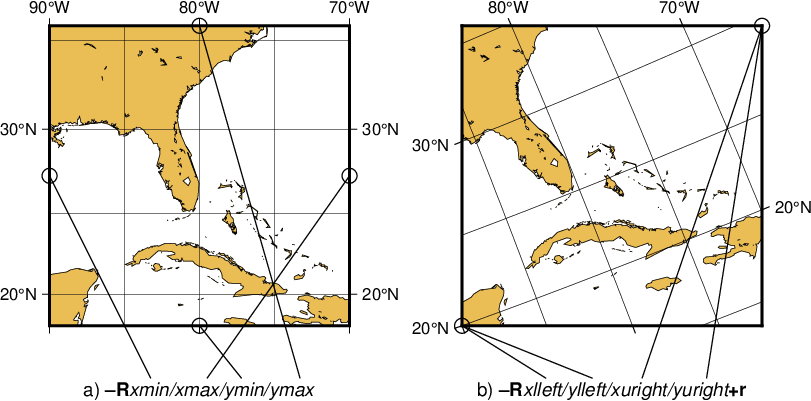
The plot region can be specified in two different ways. (a) Extreme values for each dimension, or (b) coordinates of lower left and upper right corners.
Here is the source script for the figure above:
gmt begin GMT_-R
	gmt set GMT_THEME cookbook
	gmt set MAP_FRAME_TYPE PLAIN FONT_ANNOT_PRIMARY 8p,Helvetica MAP_TICK_LENGTH_PRIMARY 0.05i \
		PS_CHAR_ENCODING ISOLatin1+
	gmt coast -R-90/-70/18/35.819 -JM2i -Dl -Glightbrown -Wthinnest -Ba10g5 -BWsEN
	gmt text -R0/2/-0.5/2 -Jx1i -N -Y-0.5i -F+f9p,Helvetica-Oblique+jCT << EOF
1	-0.375	@%0%a)@%% @%1%\035R@%%xmin/xmax/ymin/ymax
EOF
	gmt plot -N -Sc0.1i -Wthinner << EOF
0	1
1	0
1	2
2	1
EOF
	gmt plot -N -Wthinner << EOF
>
0	1
0.675	-0.35
>
1	0
1.28	-0.35
>
1	2
1.67	-0.35
>
2	1
1.05	-0.35
EOF
	gmt coast -R-90/20/-65.5327/29.4248+r -JOc280/20/22/69/2i -Dl -Glightbrown -Wthinnest -Ba10g5 -BWsEN -X2.75i -Y0.5i
	gmt text -R0/2/-0.5/2 -Jx1i -N -Y-0.5i -F+f9p,Helvetica-Oblique+jCT << EOF
1	-0.375	@%0%b)@%% @%1%\035R@%%xlleft/ylleft/xuright/yuright@%1%+r@%%
EOF
	gmt plot -N -Sc0.1i -Wthinner << EOF
0	0
2	2
EOF
	gmt plot -N -Wthinner << EOF
>
0	0
0.56	-0.35
>
0	0
0.87	-0.35
>
2	2
1.2	-0.35
>
2	2
1.63	-0.35
EOF
gmt end show
4.2. Coordinate transformations and map projections: The -J option
This option selects the coordinate transformation or map projection. The general format is
-J\(\delta\)[parameters/]scale. Here, \(\delta\) is a lower-case letter of the alphabet that selects a particular map projection, the parameters is zero or more slash-delimited projection parameter, and scale is map scale given in plot-units /degree or as 1:xxxxx.
-J\(\Delta\)[parameters/]width. Here, \(\Delta\) is an upper-case letter of the alphabet that selects a particular map projection, the parameters is zero or more slash-delimited projection parameter, and width is map width in plot-units (map height is automatically computed from the implied map scale and region).
Since GMT version 4.3.0, there is an alternative way to specify the projections: use the same abbreviation as in the mapping package PROJ. The options thus either look like:
-Jabbrev/[parameters/]scale. Here, abbrev is a lower-case abbreviation that selects a particular map projection, the parameters is zero or more slash-delimited projection parameter, and scale is map scale given in distance units per degree or as 1:xxxxx.
-JAbbrev/[parameters/]width. Here, Abbrev is an capitalized abbreviation that selects a particular map projection, the parameters is zero or more slash-delimited projection parameter, and width is map width (map height is automatically computed from the implied map scale and region).
The over 30 map projections and coordinate transformations available in GMT are represented in the Figure GMT Projections.
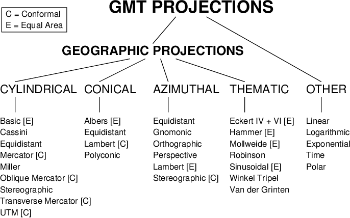
The over-30 map projections and coordinate transformations available in GMT
Here is the source script for the figure above:
gmt begin GMT_-J
	gmt set GMT_THEME cookbook
	gmt text -R0/5/0/3 -Jx1i -F+f+j << EOF
2.5	2.8	16p,Helvetica-Bold	BC	GMT PROJECTIONS
2	2.25	12p,Helvetica-Bold	BC	GEOGRAPHIC PROJECTIONS
0	1.75	11p,Helvetica		BL	CYLINDRICAL
1.1	1.75	11p,Helvetica		BL	CONICAL
2	1.75	11p,Helvetica		BL	AZIMUTHAL
3	1.75	11p,Helvetica		BL	THEMATIC
4	1.75	11p,Helvetica		BL	OTHER
EOF
	gmt text -F+f8p+jBL << EOF
0	1.35	Basic [E]
0	1.2	Cassini
0	1.05	Equidistant
0	0.9	Mercator [C]
0	0.75	Miller
0	0.6	Oblique Mercator [C]
0	0.45	Stereographic
0	0.3 	Transverse Mercator [C]
0	0.15	UTM [C]
1.1	1.35	Albers [E]
1.1	1.2	Equidistant
1.1	1.05	Lambert [C]
1.1	0.9	Polyconic
2	1.35	Equidistant
2	1.2	Gnomonic
2	1.05	Orthographic
2	0.9	Perspective
2	0.75	Lambert [E]
2	0.6	Stereographic [C]
3	1.35	Eckert IV + VI [E]
3	1.2	Hammer [E]
3	1.05	Mollweide [E]
3	0.9	Robinson
3	0.75	Sinusoidal [E]
3	0.6	Winkel Tripel
3	0.45	Van der Grinten
4	1.35	Linear
4	1.2	Logarithmic
4	1.05	Exponential
4	0.9	Time
4	0.75	Polar
0.075	2.75	C = Conformal
0.075	2.6	E = Equal Area
EOF

	gmt plot -Wthinner << EOF
>
2.3	2.75
2	2.4
>
2.7	2.75
4.2	1.9
>
1.7	2.2
0.2	1.9
>
1.9	2.2
1.3	1.9
>
2.1	2.2
2.2	1.9
>
2.3	2.2
3.2	1.9
>
0.2	1.7
0.2	1.5
>
1.3	1.7
1.3	1.5
>
2.2	1.7
2.2	1.5
>
3.2	1.7
3.2	1.5
>
4.2	1.7
4.2	1.5
>
0.025	2.55
0.875	2.55
0.875	2.87
0.025	2.87
0.025	2.55
EOF
gmt end show
4.2.1. Projections specifications
GMT offers 31 map projections specified using the -J option. There are two conventions you may use: (a) GMT-style syntax and (b) PROJ-style syntax. The codes for the GMT-style and the PROJ-style are tabulated below along with the associated parameters and links to the cookbook sections that describe the projection syntax and usage.
Projection |
GMT CODES |
PROJ CODES |
Parameters |
|---|---|---|---|
-J (scale|WIDTH); |
-J (scale) |
||
-Ja|A |
-Jlaea/ |
lon0/lat0[/horizon]/scale|width |
|
-Jb|B |
-Jaea/ |
lon0/lat0/lat1/lat2/scale|width |
|
-Jc|C |
-Jcass/ |
lon0/lat0/scale|width |
|
-Jcyl_stere|Cyc_stere |
-Jcyl_stere/ |
[lon0[/lat0]/]scale|width |
|
-Jd|D |
-Jeqdc/ |
lon0/lat0/lat1/lat2/scale|width |
|
-Je|E |
-Jaeqd/ |
lon0/lat0[/horizon]/scale|width |
|
-Jf|F |
-Jgnom/ |
lon0/lat0[/horizon]/scale|width |
|
-Jg|G |
-Jortho/ |
lon0/lat0[/horizon]/scale|width |
|
-Jg|G |
-Jnsper/ |
lon0/lat0/scale|width[+aazimuth][+ttilt][+vvwidth/vheight][+wtwist][+zaltitude[r|R]|g] |
|
-Jh|H |
-Jhammer/ |
lon0/scale|width |
|
-Ji|I |
-Jsinu/ |
lon0/scale|width |
|
-Jj|J |
-Jmill/ |
lon0/scale|width |
|
-Jkf|Kf |
-Jeck4/ |
lon0/scale|width |
|
-Jks|Ks |
-Jeck6/ |
lon0/scale|width |
|
-Jl|L |
-Jlcc/ |
lon0/lat0/lat1/lat2/scale|width |
|
-Jm|M |
-Jmerc/ |
[lon0[/lat0/]]scale|width |
|
-Jn|N |
-Jrobin/ |
[lon0/]scale|width |
|
-Jo|O[a|A] |
-Jomerc/ |
lon0/lat0/azim/scale|width [+v] |
|
-Jo|O[b|B] |
-Jomerc/ |
lon0/lat0/lon1/lat1/scale|width[+v] |
|
-Jo|O[c|C] |
-Jomercp/ |
lon0/lat0/lonp/latp/scale|width[+v] |
|
Polar [azimuthal] (\(\theta, r\)) (or cylindrical) |
-Jp|P |
-Jpolar/ |
scale|width[+a][+f[e|p|radius]][+kkind][+roffset][+torigin][+z[p|radius]] |
-Jpoly|Poly |
-Jpoly/ |
[lon0[/lat0/]]scale|width |
|
-Jq|Q |
-Jeqc/ |
[lon0[/lat0/]]scale|width |
|
-Jr|R |
-Jwintri/ |
[lon0/]scale|width |
|
-Js|S |
-Jstere/ |
lon0/lat0[/horizon]/scale|width |
|
-Jt|T |
-Jtmerc/ |
[lon0[/lat0/]]scale|width |
|
-Ju|U |
-Jutm/ |
zone/scale|width |
|
-Jv|V |
-Jvandg/ |
[lon0/]scale|width |
|
-Jw|W |
-Jmoll/ |
[lon0/]scale|width |
|
Linear, logarithmic, power, and time |
-Jx|X |
-Jxy |
xscale|width[l|ppower|T|t][/yscale|height[l|ppower|T|t]][d] |
-Jy|Y |
-Jcea/ |
lon0/lat0/scale|width |
4.3. Map frame and axes annotations: The -B option
Syntax
- -B[p|s]parameters
Set map boundary frame and axes attributes.
Description
This is potentially the most complicated option in GMT, but most examples of its usage are actually quite simple. We distinguish between two sets of information: Frame settings and Axes settings. These are set separately by their own -B invocations; hence multiple -B specifications may be specified. The Frame settings cover things such as which axes should be plotted, canvas fill, plot title (and subtitle), and what type of gridlines be drawn, whereas the Axes settings deal with annotation, tick, and gridline intervals, axes labels, and annotation units.
4.3.1. Frame settings
The Frame settings are specified by
-B[axes][+b][+gfill][+i[val]][+n][+olon/lat][+ssubtitle][+ttitle][+w[pen]][+xfill][+yfill][+zfill]
The frame setting is optional but can be invoked once to override the defaults. The following modifiers can be appended to -B to control the Frame settings:
axes to set which of the axes should be drawn and possibly annotated using a combination of the codes listed below [default is theme dependent]. Borders omitted from the set of codes will not be drawn. For example, WSn denotes that the “western” (left) and “southern” (bottom) axes should be drawn with tick-marks and annotations by using W and S; that the “northern” (top) edge of the plot should be drawn with tick-marks and without annotations by using n; and that the “eastern” (right) axes should not be drawn by not including one of E|e|r.
West, East, South, North, and/or (for 3-D plots) Z indicate axes that should be drawn with both tick-marks and annotations.
west, east, south, north, and/or (for 3-D plots) z indicate axes that should be drawn with tick-marks but without annotations.
l(eft), r(ight), b(ottom), t(op) and/or (for 3-D plots) u(p) indicate axes that should be drawn without tick-marks or annotations.
Z|zcode (for 3-D plots) where code is any combination of the corner ids 1, 2, 3, 4. By default, a single vertical axes will be plotted for 3-D plots at the most suitable map corner. code can be used to override this, where 1 represents the south-western (lower-left) corner, 2 the south-eastern (lower-right), 3 the north-eastern (upper-right), and 4 the north-western (upper-left) corner.
+w[pen] (for 3-D plots) to draw the outlines of the x-z and y-z planes [default is no outlines]. Optionally, append pen to specify different pen attributes [default is MAP_GRID_PEN_PRIMARY].
+b (for 3-D plots) to draw the foreground lines of the 3-D cube defined by -R.
+gfill to paint the interior of the canvas with a color specified by fill [default is no fill]. This also sets fill for the two back-walls in 3-D plots.
+xfill to paint the yz plane with a color specified by fill [default is no fill].
+yfill to paint the xz plane with a color specified by fill [default is no fill].
+zfill to paint the xy plane with a color specified by fill [default is no fill].
+i[val] to annotate an internal meridian or parallel when the axis that normally would be drawn and annotated does not exist (e.g., for an azimuthal map with 360-degree range that has no latitude axis or a global Hammer map that has no longitude axis). val gives the meridian or parallel that should be annotated [default is 0].
+olon/lat to produce oblique gridlines about another pole specified by lon/lat [default references to the North pole]. +o is ignored if no gridlines are requested.
+n to have no frame and annotations at all [default is contolled by axes].
+ttitle to place the string given in title centered above the plot frame [default is no title].
+ssubtitle (requires +ttitle) to place the string given in subtitle beneath the title [default is no subtitle].
Note: Both +ttitle and +ssubtitle may be set over multiple lines by breaking them up using the
markers @^ or <break>. To include LaTeX code as part of a single-line title or subtitle, enclose the expression
with @[ markers (or alternatively <math> … </math>) (requires latex and dvips to be installed). See the
Using LaTeX Expressions in GMT chapter for more details.
4.3.2. Axes settings
The Axes settings are specified by
-B[p|s][x|y|z]intervals[+aangle|n|p][+f][+llabel][+pprefix][+uunit]
but you may also split this into two separate invocations for clarity, i.e.,
-B[p|s][x|y|z][+aangle|n|p][+e[l|u]][+f][+l|Llabel][+pprefix][+s|Sseclabel][+uunit]-B[p|s][x|y|z]intervals
The following modifiers can be appended to -B to control the Axes settings:
p|s to set whether the modifiers apply to the p(rimary) or s(econdary) axes [Default is p]. These settings are mostly used for time axes annotations but are available for geographic axes as well. Note: Primary refers to annotations closest to the axis and secondary to annotations further away. Hence, primary annotation-, tick-, and gridline-intervals must be shorter than their secondary counterparts. The terms “primary” and “secondary” do not reflect any hierarchical order of units: the “primary” annotation interval is usually smaller (e.g., days) while the “secondary” annotation interval typically is larger (e.g., months).
x|y|z to set which axes the modifiers apply to [default is xy]. If you wish to give different annotation intervals or labels for the various axes then you must repeat the B option for each axis. For a 3-D plot with the -p and -Jz options used, -Bz can be used to provide settings for the vertical axis.
+e to give skip annotations that fall exactly at the ends of the axis. Append l or u to only skip the lower or upper annotation, respectively.
+f (for geographic axes only) to give fancy annotations with W|E|S|N suffices encoding the sign.
+l|+Llabel (for Cartesian plots only) to add a label to an axis. +l uses the default label orientation; +L forces a horizontal label for y-axes, which is useful for very short labels.
+s|Sseclabel (for Cartesion plots only) to specify an alternate label for the right or upper axes. +s uses the default label orientation; +S forces a horizontal label for y-axes, which is useful for very short labels.
+pprefix (for Cartesion plots only) to define a leading text prefix for the axis annotation (e.g., dollar sign for plots related to money). For geographic maps the addition of degree symbols, etc. is automatic and controlled by FORMAT_GEO_MAP.
+uunit (for Cartesion plots only) to append specific units to the annotations. For geographic maps the addition of degree symbols, etc. is automatic and controlled by FORMAT_GEO_MAP.
+aangle (for Cartesion plots only) to plot slanted annotations, where angle is measured with respect to the horizontal and must be in the -90 <= angle <= 90 range. +an can be used as a shorthand for normal (i.e., +a90) [Default for y-axis] and +ap for parallel (i.e., +a0) annotations [Default for x-axis]. These defaults can be changed via MAP_ANNOT_ORTHO.
intervals to define the intervals for annotations and major tick spacing, minor tick spacing, and/or grid line spacing. See Intervals Specification for the formatting associated with this modifier.
NOTE: To include LaTeX code as part of a label, enclose the expression with @[ markers (or alternatively <math>
… </math>). (requires latex and dvips to be installed). See the Using LaTeX Expressions in GMT chapter for more
details.
NOTE: If any labels, prefixes, or units contain spaces or special characters you will need to enclose them in quotes.
NOTE: Text items such as title, subtitle, label and seclabel are seen by GMT as part of a long string containing everything passed to -B. Therefore, they cannot contain substrings that look like other modifiers. If you need to embed such sequences (e.g., +t“Solving a+b=c”) you need to replace those + symbols with their octal equivalent \053, (e.g., +t“Solving a\053b=c”).
NOTE: For non-geographical projections: Give negative scale (in -Jx) or axis length (in -JX) to change the direction of increasing coordinates (i.e., to make the y-axis positive down).
[a|f|g][stride][phase][unit].
The choice of a|f|g sets the axis item of interest, which are detailed in the Table interval types. Optionally, append phase to shift the annotations by that amount (positive or negative with the sign being required). Optionally, append unit to specify the units of stride, where unit is one of the 18 supported unit codes. For custom annotations and intervals, intervals can be given as cintfile, where intfile contains any number of records with coord type [label]. See the section Custom axes for more details.
Flag |
Description |
|---|---|
a |
Annotation and major tick spacing |
f |
Minor tick spacing |
g |
Grid line spacing |
NOTE: The appearance of certain time annotations (month-, week-, and day-names) may be affected by the GMT_LANGUAGE, FORMAT_TIME_PRIMARY_MAP, and FORMAT_TIME_SECONDARY_MAP settings.
Automatic intervals: GMT will auto-select the spacing between the annotations and major ticks, minor ticks, and grid lines if stride is not provided after a|f|g. This can be useful for automated plots where the region may not always be the same, making it difficult to determine the appropriate stride in advance. For example, -Bafg will select all three spacings automatically for both axes. In case of longitude–latitude plots, this will keep the spacing the same on both axes. You can also use -Bxafg -Byafg to auto-select them separately. Note that given the myriad ways of specifying time-axis annotations, the automatic selections may need to be overridden with manual settings to achieve exactly what you need. When stride is omitted after g, the grid line are spaced the same as the minor ticks; unless g is used in consort with a, in which case the grid lines are spaced the same as the annotations.
Stride units: The unit flag can take on one of 18 codes which are listed in Table Units. Almost all of these units are time-axis specific. However, the d, m, and s units will be interpreted as arc degrees, minutes, and arc seconds respectively when a map projection is in effect.
Flag |
Unit |
Description |
|---|---|---|
Y |
year |
Plot using all 4 digits |
y |
year |
Plot using last 2 digits |
O |
month |
Format annotation using FORMAT_DATE_MAP |
o |
month |
Plot as 2-digit integer (1–12) |
U |
ISO week |
Format annotation using FORMAT_DATE_MAP |
u |
ISO week |
Plot as 2-digit integer (1–53) |
r |
Gregorian week |
7-day stride from start of week (see TIME_WEEK_START) |
K |
ISO weekday |
Plot name of weekday in selected language |
k |
weekday |
Plot number of day in the week (1–7) (see TIME_WEEK_START) |
D |
date |
Format annotation using FORMAT_DATE_MAP |
d |
day |
Plot day of month (1–31) or day of year (1–366) (see FORMAT_DATE_MAP) |
R |
day |
Same as d; annotations aligned with week (see TIME_WEEK_START) |
H |
hour |
Format annotation using FORMAT_CLOCK_MAP |
h |
hour |
Plot as 2-digit integer (0–24) |
M |
minute |
Format annotation using FORMAT_CLOCK_MAP |
m |
minute |
Plot as 2-digit integer (0–60) |
S |
seconds |
Format annotation using FORMAT_CLOCK_MAP |
s |
seconds |
Plot as 2-digit integer (0–60) |
NOTE: If your axis is in radians you can use multiples or fractions of pi to set such annotation intervals. The format is [s]pi[f], for an optional integer scale s and optional integer fraction f. When GMT parses one of these forms we alert the labeling machinery to look for certain combinations of pi, limited to npi, 3/2 pi (3pi2), and fractions 3/4 (3pi4), 2/3 (2pi3), 1/2 (1pi2), 1/3 (1pi3), and 1/4 (1pi4) in the interval given to the -B axes settings. When an annotated value is within roundoff-error of these combinations we typeset the label using the Greek letter \(\pi\) and required multiples or fractions.
- NOTE: These GMT parameters can affect the appearance of the map boundary:
MAP_ANNOT_MIN_ANGLE, MAP_ANNOT_MIN_SPACING, FONT_ANNOT_PRIMARY, FONT_ANNOT_SECONDARY, MAP_ANNOT_OFFSET_PRIMARY, MAP_ANNOT_OFFSET_SECONDARY, MAP_ANNOT_ORTHO, MAP_FRAME_AXES, MAP_DEFAULT_PEN, MAP_FRAME_TYPE, FORMAT_GEO_MAP, MAP_FRAME_PEN, MAP_FRAME_WIDTH, MAP_GRID_CROSS_SIZE_PRIMARY, MAP_GRID_PEN_PRIMARY, MAP_GRID_CROSS_SIZE_SECONDARY, MAP_GRID_PEN_SECONDARY, FONT_TITLE, FONT_LABEL, MAP_LINE_STEP, MAP_ANNOT_OBLIQUE, FORMAT_CLOCK_MAP, FORMAT_DATE_MAP, FORMAT_TIME_PRIMARY_MAP, FORMAT_TIME_SECONDARY_MAP, GMT_LANGUAGE, TIME_WEEK_START, MAP_TICK_LENGTH_PRIMARY, and MAP_TICK_PEN_PRIMARY; see the gmt.conf man page for details.
4.3.3. Geographic basemaps
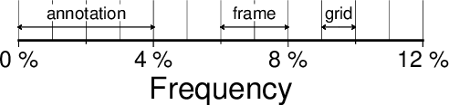
Geographic basemaps may differ from regular plot axis in that some projections support a “fancy” form of axis and is selected by the MAP_FRAME_TYPE setting. The annotations will be formatted according to the FORMAT_GEO_MAP template and MAP_DEGREE_SYMBOL setting. A simple example of part of a basemap is shown in Figure Geographic map border.
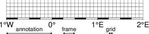
Geographic map border using separate selections for annotation, frame, and grid intervals. Formatting of the annotation is controlled by the parameter FORMAT_GEO_MAP in your gmt.conf.
Here is the source script for the figure above:
gmt begin GMT_-B_geo_1
	gmt set GMT_THEME cookbook
	gmt set FORMAT_GEO_MAP ddd:mm:ssF
	gmt basemap -R-1/2/0/0.4 -JM3i -Ba1f15mg5m -BS
	gmt plot -Sv2p+e+a60 -W0.5p -Gblack -Y-0.35i -N << EOF
-0.5 0 0 0.5
-0.5 0 180 0.5
0.375 0 0 0.125
0.375 0 180 0.125
1.29166666 0 0 0.04166666
1.29166666 0 180 0.04166666
EOF
	gmt text -F+f9p+jCB << EOF
-0.5 0.05 annotation
0.375 0.05 frame
1.29166666 0.05 grid
EOF
gmt end show
The machinery for primary and secondary annotations introduced for time-series axes can also be utilized for geographic basemaps. This may be used to separate degree annotations from minutes- and seconds-annotations. For a more complicated basemap example using several sets of intervals, including different intervals and pen attributes for grid lines and grid crosses, see Figure Complex basemap.
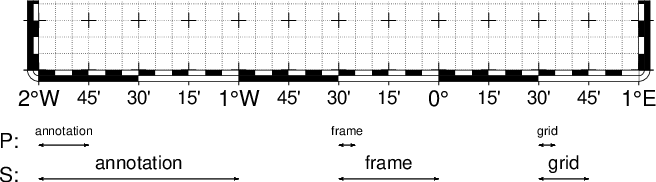
Geographic map border with both primary (P) and secondary (S) components.
Here is the source script for the figure above:
gmt begin GMT_-B_geo_2
	gmt set GMT_THEME cookbook
	gmt set FORMAT_GEO_MAP ddd:mm:ssF FONT_ANNOT_PRIMARY +9p
	gmt basemap -R-2/1/0/0.35 -JM4i -Bpa15mf5mg5m -BwSe -Bs1f30mg15m --MAP_FRAME_TYPE=fancy-rounded \
		--MAP_GRID_PEN_PRIMARY=thinnest,black,. --MAP_GRID_CROSS_SIZE_SECONDARY=0.1i \
		--MAP_FRAME_WIDTH=0.075i --MAP_TICK_LENGTH_PRIMARY=0.1i
	gmt plot -Sv0.03i+b+e+jc -W0.5p -Gblack -Y-0.5i -N << EOF
-1.875 0 0 0.33333
-0.45833 0 0 0.11111
0.541666 0 0 0.11111
EOF
	gmt text -N -F+f+j << EOF
-2.1 0.025 10p RM P:
-1.875 0.05 6p CB annotation
-0.45833 0.05 6p CB frame
0.541666 0.05 6p CB grid
EOF
	gmt plot -Sv0.03i+b+e+jc -W0.5p -Gblack -Y-0.225i -N << EOF
-1.5 0 0 1.33333
-0.25 0 0 0.66666
0.625 0 0 0.33333
EOF
	gmt text -N -F+f+j << EOF
-2.1 0.025 10p RM S:
-1.5  0.05 9p CB annotation
-0.25 0.05 9p CB frame
0.625 0.05 9p CB grid
EOF
gmt end show
4.3.4. Cartesian linear axes
For non-geographic axes, the MAP_FRAME_TYPE setting is implicitly set to plain. Other than that, cartesian linear axes are very similar to geographic axes. The annotation format may be controlled with the FORMAT_FLOAT_OUT parameter. By default, it is set to “%g”, which is a C language format statement for floating point numbers [13], and with this setting the various axis routines will automatically determine how many decimal points should be used by inspecting the stride settings. If FORMAT_FLOAT_OUT is set to another format it will be used directly (e.g., “%.2f” for a fixed, two decimals format). Note that for these axes you may use the unit setting to add a unit string to each annotation (see Figure Axis label).
Linear Cartesian projection axis. Long tick-marks accompany
annotations, shorter ticks indicate frame interval. The axis label is
optional. For this example we used -R0/12/0/0.95 -JX7.5c/0.75c -Ba4f2g1+lFrequency+u" %" -BS
Here is the source script for the figure above:
gmt begin GMT_-B_linear
	gmt set GMT_THEME cookbook
	gmt basemap -R0/12/0/0.95 -JX7.5c/0.75c -Ba4f2g1+lFrequency+u" %" -BS
	gmt plot -Sv2p+e+a60 -W0.5p -Gblack -Y0.25c -N << EOF
2 0 0 0.5
2 0 180 0.5
7 0 0 0.25
7 0 180 0.25
9.5 0 0 0.125
9.5 0 180 0.125
EOF
	gmt text -Gwhite -C1p -F+f9p+jCB << EOF
2 0.2 annotation
7 0.2 frame
9.5 0.2 grid
EOF
gmt end show
There are occasions when the length of the annotations are such that placing them horizontally (which is the default) may lead to overprinting or too few annotations. One solution is to request slanted annotations for the x-axis (e.g., Figure Axis label) via the +aangle modifier.

Linear Cartesian projection axis with slanted annotations.
For this example we used -R2000/2020/35/45 -JX12c -Bxa2f+a-30 -BS.
For the y-axis only the modifier +ap for parallel is allowed.
Here is the source script for the figure above:
gmt basemap -R2000/2020/35/45 -JX12c -Bxa2f+a-30 -BS --GMT_THEME=cookbook -view GMT_-B_slanted
4.3.5. Cartesian log10 axes
Due to the logarithmic nature of annotation spacings, the stride parameter takes on specific meanings. The following concerns are specific to log axes (see Figure Logarithmic projection axis):
stride must be 1, 2, 3, or a negative integer -n. Annotations/ticks will then occur at 1, 1-2-5, or 1,2,3,4,…,9, respectively, for each magnitude range. For -n the annotations will take place every n‘th magnitude.
Append l to stride. Then, log10 of the annotation is plotted at every integer log10 value (e.g., x = 100 will be annotated as “2”) [Default annotates x as is].
Append p to stride. Then, annotations appear as 10 raised to log10 of the value (e.g., 10-5).
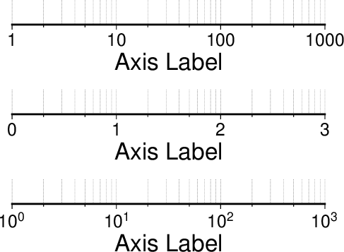
Logarithmic projection axis using separate values for annotation, frame, and grid intervals. (top) Here, we have chosen to annotate the actual values. Interval = 1 means every whole power of 10, 2 means 1, 2, 5 times powers of 10, and 3 means every 0.1 times powers of 10. We used -R1/1000/0/1 -JX7.5cl/0.6c -Ba1f2g3. (middle) Here, we have chosen to annotate \(\log_{10}\) of the actual values, with -Ba1f2g3l. (bottom) We annotate every power of 10 using \(\log_{10}\) of the actual values as exponents, with -Ba1f2g3p.
Here is the source script for the figure above:
gmt begin GMT_-B_log
	gmt set GMT_THEME cookbook
	gmt set MAP_GRID_PEN_PRIMARY thinnest,.
	gmt basemap -R1/1000/0/1 -JX7.5cl/0.6c -B1f2g3p+l"Axis Label" -BS
	gmt basemap -B1f2g3l+l"Axis Label" -BS -Y2.15c
	gmt basemap -B1f2g3+l"Axis Label" -BS -Y2.15c
gmt end show
4.3.6. Cartesian exponential axes
Normally, stride will be used to create equidistant (in the user’s unit) annotations or ticks, but because of the exponential nature of the axis, such annotations may converge on each other at one end of the axis. To avoid this problem, you can append p to stride, and the annotation interval is expected to be in transformed units, yet the annotation itself will be plotted as un-transformed units (see Figure Power projection axis). E.g., if stride = 1 and power = 0.5 (i.e., sqrt), then equidistant annotations labeled 1, 4, 9, … will appear.
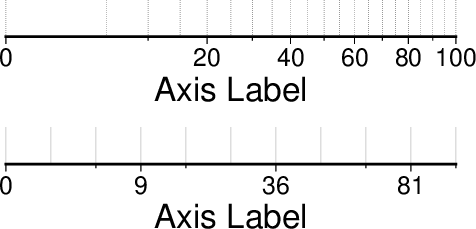
Exponential or power projection axis. (top) Using an exponent of 0.5 yields a \(sqrt(x)\) axis. Here, intervals refer to actual data values, in -R0/100/0/0.9 -JX3ip0.5/0.25i -Ba20f10g5. (bottom) Here, intervals refer to projected values, although the annotation uses the corresponding unprojected values, as in -Ba3f2g1p.
Here is the source script for the figure above:
gmt begin GMT_-B_pow
	gmt set GMT_THEME cookbook
	gmt set MAP_GRID_PEN_PRIMARY thinnest,.
	gmt basemap -R0/100/0/0.9 -JX3ip0.5/0.25i -Ba3f2g1p+l"Axis Label" -BS
	gmt basemap -Ba20f10g5+l"Axis Label" -BS -Y0.85i
gmt end show
4.3.7. Cartesian time axes
What sets time axis apart from the other kinds of plot axes is the numerous ways in which we may want to tick and annotate the axis. Not only do we have both primary and secondary annotation items but we also have interval annotations versus tick-mark annotations, numerous time units, and several ways in which to modify the plot. We will demonstrate this flexibility with a series of examples. While all our examples will only show a single x-axis (south, selected via -BS), time-axis annotations are supported for all axes.
Our first example shows a time period of almost two months in Spring 2000. We want to annotate the month intervals as well as the date at the start of each week:
gmt begin GMT_-B_time1
	gmt set GMT_THEME cookbook
	gmt set FORMAT_DATE_MAP=-o FONT_ANNOT_PRIMARY +9p
	gmt basemap -R2000-4-1T/2000-5-25T/0/1 -JX12c/0.5c -Bpxa7Rf1d -Bsxa1O -BS
gmt end show
These commands result in Figure Cartesian time axis. Note the leading hyphen in the FORMAT_DATE_MAP removes leading zeros from calendar items (e.g., 02 becomes 2).

Cartesian time axis, example 1
The next example shows two different ways to annotate an axis portraying 2 days in July 1969:
gmt begin GMT_-B_time2
	gmt set GMT_THEME cookbook
  gmt set FORMAT_DATE_MAP "o dd" FORMAT_CLOCK_MAP hh:mm FONT_ANNOT_PRIMARY +9p
  gmt basemap -R1969-7-21T/1969-7-23T/0/1 -JX12c/0.5c -Bpxa6Hf1h -Bsxa1K -BS
  gmt basemap -Bpxa6Hf1h -Bsxa1D -BS -Y1.6c
gmt end show
The lower example (Figure Cartesian time axis, example 2) chooses to annotate the weekdays (by specifying a1K) while the upper example choses dates (by specifying a1D). Note how the clock format only selects hours and minutes (no seconds) and the date format selects a month name, followed by one space and a two-digit day-of-month number.
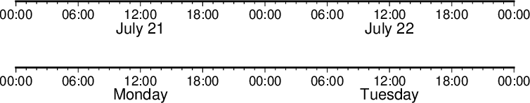
Cartesian time axis, example 2
The third example (Figure Cartesian time axis, example 3) presents two years, annotating both the years and every 3rd month.
gmt begin GMT_-B_time3
	gmt set GMT_THEME cookbook
	gmt set FORMAT_DATE_MAP o FORMAT_TIME_PRIMARY_MAP Character FONT_ANNOT_PRIMARY +9p
	gmt basemap -R1997T/1999T/0/1 -JX12c/0.5c -Bpxa3Of1o -Bsxa1Y -BS
gmt end show
Note that while the year annotation is centered on the 1-year interval, the month annotations must be centered on the corresponding month and not the 3-month interval. The FORMAT_DATE_MAP selects month name only and FORMAT_TIME_PRIMARY_MAP selects the 1-character, upper case abbreviation of month names using the current language (selected by GMT_LANGUAGE).

Cartesian time axis, example 3
The fourth example (Figure Cartesian time axis, example 4) only shows a few hours of a day, using relative time by specifying t in the -R option while the TIME_UNIT is d (for days). We select both primary and secondary annotations, ask for a 12-hour clock, and let time go from right to left:
gmt begin GMT_-B_time4
	gmt set GMT_THEME cookbook
	gmt set FORMAT_CLOCK_MAP=-hham FONT_ANNOT_PRIMARY +9p TIME_UNIT d
	gmt basemap -R0.2t/0.35t/0/1 -JX-12c/0.5c -Bpxa15mf5m -Bsxa1H -BS
gmt end show

Cartesian time axis, example 4
The fifth example shows a few weeks of time (Figure Cartesian time axis, example 5). The lower axis shows ISO weeks with week numbers and abbreviated names of the weekdays. The upper uses Gregorian weeks (which start at the day chosen by TIME_WEEK_START); they do not have numbers.
gmt begin GMT_-B_time5
	gmt set GMT_THEME cookbook
	gmt set FORMAT_DATE_MAP u FORMAT_TIME_PRIMARY_MAP Character FORMAT_TIME_SECONDARY_MAP full FONT_ANNOT_PRIMARY +9p
	gmt basemap -R1969-7-21T/1969-8-9T/0/1 -JX12c/0.5c -Bpxa1K -Bsxa1U -BS
	gmt set FORMAT_DATE_MAP o TIME_WEEK_START Sunday FORMAT_TIME_SECONDARY_MAP Character
	gmt basemap -Bpxa3Kf1k -Bsxa1r -BS -Y1.6c
gmt end show
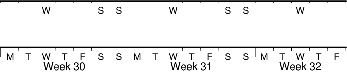
Cartesian time axis, example 5
Our sixth example (Figure Cartesian time axis, example 6) shows the first five months of 1996, and we have annotated each month with an abbreviated, upper case name and 2-digit year. Only the primary axes information is specified.
gmt begin GMT_-B_time6
	gmt set GMT_THEME cookbook
	gmt set FORMAT_DATE_MAP "o yy" FORMAT_TIME_PRIMARY_MAP Abbreviated
	gmt basemap -R1996T/1996-6T/0/1 -JX12c/0.5c -Bxa1Of1d -BS
gmt end show

Cartesian time axis, example 6
Our seventh and final example (Figure Cartesian time axis, example 7) illustrates annotation of year-days. Unless we specify the formatting with a leading hyphen in FORMAT_DATE_MAP we get 3-digit integer days. Note that in order to have the two years annotated we need to allow for the annotation of small fractional intervals; normally such truncated interval must be at least half of a full interval.
gmt begin GMT_-B_time7
	gmt set GMT_THEME cookbook
	gmt set FORMAT_DATE_MAP jjj TIME_INTERVAL_FRACTION 0.05 FONT_ANNOT_PRIMARY +9p
	gmt basemap -R2000-12-15T/2001-1-15T/0/1 -JX12c/0.5c -Bpxa5Df1d -Bsxa1Y -BS
gmt end show

Cartesian time axis, example 7
4.3.8. Custom axes
Irregularly spaced annotations or annotations based on look-up tables can be implemented using the custom annotation mechanism. Here, we given the c (custom) type to the -B option followed by a filename that contains the annotations (and tick/grid-lines specifications) for one axis. The file can contain any number of comments (lines starting with #) and any number of records of the format
The coord is the location of the desired annotation, tick, or grid-line, whereas type is a string composed of letters from a (annotation), i interval annotation, f frame tick, and g gridline. You must use either a or i within one file; no mixing is allowed. The coordinates should be arranged in increasing order. If label is given it replaces the normal annotation based on the coord value. Our last example (Figure Custom and irregular annotations) shows such a custom basemap with an interval annotations on the x-axis and irregular annotations on the y-axis.
cat << EOF >| xannots.txt
416.0	ig	Devonian
443.7	ig	Silurian
488.3	ig	Ordovician
542	ig	Cambrian
EOF
cat << EOF >| yannots.txt
0	a
1	a
2	f
2.71828	ag	e
3	f
3.1415926	ag	@~p@~
4	f
5	f
6	f
6.2831852	ag	2@~p@~
EOF

gmt begin GMT_-B_custom
	gmt set GMT_THEME cookbook
	gmt basemap -R416/542/0/6.2831852 -JX-12c/6c -Bpx25f5g25+u" Ma" -Bpycyannots.txt -Bsxcxannots.txt -BWS+glightblue \
		--MAP_ANNOT_OFFSET_SECONDARY=10p --MAP_GRID_PEN_SECONDARY=2p
gmt end show
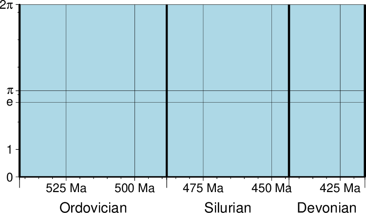
Custom and irregular annotations, tick-marks, and gridlines.
4.4. Timestamps on plots: The -U option
Syntax
- -U[label|+c][+jjust][+odx[/dy]]
Draw GMT time stamp logo on plot.
Description
The -U option draws the GMT system time stamp on the plot. The following modifiers are supported:
label to append the text string given in label (which must be surrounded by double quotes if it contains spaces).
+c to plot the current command string.
+jjustify to specify the justification of the time stamp, where justify is a two-character justification code that is a combination of a horizontal (L(eft), C(enter), or R(ight)) and a vertical (T(op), M(iddle), or B(ottom)) code [default is BL].
+odx[/dy] to offset the anchor point for the time stamp by dx and optionally dy (if different than dx).
The GMT parameters MAP_LOGO, MAP_LOGO_POS, FONT_LOGO and FORMAT_TIME_STAMP can affect the appearance; see the gmt.conf man page for details. The time string will be in the locale set by the environment variable TZ (generally local time).
Examples

The -U option makes it easy to date a plot.
Here is the source script for the figure above:
gmt plot -R0/3/0/0.1 -Jx1i -U"optional command string or text here" -T --GMT_THEME=cookbook -view GMT_-U
4.5. Verbose feedback: The -V option
Syntax
- -V[level]
Select verbosity level [w].
Description
The -V option controls the verbosity mode, which determines which messages are sent to standard error. Choose among 7 levels of verbosity; each level adds more messages:
q - Quiet, not even fatal error messages are produced.
e - Error messages only.
w - Warnings (by default, same as running without -V)
t - Timings (report runtimes for time-intensive algorithms).
i - Informational messages (same as -V only).
c - Compatibility warnings (if compiled with backward-compatibility).
d - Debugging messages.
This option can also be set by specifying the default GMT_VERBOSE as quiet, error, warning, timing, compat, information, or debug, in order of increased verbosity [default is warning].
4.6. Plot positioning and layout: The -X -Y options
Syntax
- -X[a|c|f|r][xshift]
Shift plot origin.
- -Y[a|c|f|r][yshift]
Shift plot origin.
Description
The -X and -Y options shift the plot origin relative to the current origin by (xshift,yshift). Optionally, append the length unit (c, i, or p). Default is (MAP_ORIGIN_X, MAP_ORIGIN_Y) for new plots, which ensures that boundary annotations fit on the page. Subsequent overlays will be co-registered with the previous plot unless the origin is shifted using these options. The following modifiers are supported [default is r]:
Prepend a to shift the origin back to the original position after plotting.
Prepend c to center the plot on the center of the paper (optionally add a shift).
Prepend f to shift the origin relative to the fixed lower left.
Prepend r to move the origin relative to its current location.
When -X or -Y are used without any further arguments, the values from the last use of that option in a previous GMT command will be used. In modern mode, -X and -Y can also access the previous plot bounding box dimensions w and h and construct offsets that involve them. Thus, xshift can in general be [[±][f]w[/d]±]xoff, where optional signs, factor f and divisor d can be used to compute an offset that may be adjusted further by ±off. Similarly, yshift can in general be [[±][f]h[/d]±]yoff. For instance, to move the origin up 2 cm beyond the height of the previous plot, use -Yh+2c. To move the origin half the width to the right, use -Xw/2. Note: the previous plot bounding box refers to the last object plotted, which may be an image, logo, legend, colorbar, etc.
Examples
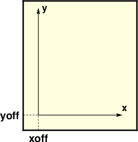
Plot origin can be translated freely with -X -Y.
Here is the source script for the figure above:
gmt begin GMT_-XY
	gmt set GMT_THEME cookbook
	gmt basemap -R0/1.5/0/1.7 -Jx1i -B0 -B+glightyellow
	gmt plot -Sv5p+e -W0.5p -Gblack << EOF
0.2	0.2	0	1.1
0.2	0.2	90	1.4
EOF
	gmt plot -Wthinnest,- << EOF
>
0	0.2
0.2	0.2
>
0.2	0
0.2	0.2
EOF
	gmt text -N --FONT=Helvetica-Bold -F+f+j << EOF
0.2	-0.05	10p	TC	xoff
-0.05	0.2	10p	RM	yoff
1.3	0.25	9p	BL	x
0.25	1.6	9p	ML	y
EOF
gmt end show
4.7. OGR/GMT GIS i/o: The -a option
Syntax
- -a[[col=]name][,…]
Control how aspatial data are handled in GMT during input and output.
Description
GMT relies on external tools to translate geospatial files such as shapefiles into a format we can read. The tool ogr2ogr in the GDAL package can do such translations and preserve the aspatial metadata via a new OGR/GMT format specification (See the cookbook chapter The GMT Vector Data Format for OGR Compatibility). For this to be useful we need a mechanism to associate certain metadata values with required input and output columns expected by GMT programs. The -a option allows you to supply one or more comma-separated associations col=name, where name is the name of an aspatial attribute field in a OGR/GMT file and whose value we wish to as data input for column col. The given aspatial field thus replaces any other value already set. Note: col = 0 is the first data column. Note: If no aspatial attributes are needed then the -a option is not needed – GMT will still process and read such data files.
4.7.1. OGR/GMT input with -a option
If you need to populate GMT data columns with (constant) values specified by aspatial attributes, use -a and append any number of comma-separated col=name associations. For example, -a2=depth will read the spatial x,y columns from the file and add a third (z) column based on the value of the aspatial field called depth. You can also associate aspatial fields with other settings such as labels, fill colors, pens, and values (for looking-up colors) by letting the col value be one of D (for distance), G (for fill), I (for ID), L (for label), T (for text), W (for pen), or Z (for value). This works analogously to how standard multi-segment files can pass such options via its segment headers (See the cookbook chapter GMT File Formats). Note: If the leading col= is omitted, the column value is automatically incremented starting at 2.
4.7.2. OGR/GMT output with -a option
GMT table-writing tools can also output the OGR/GMT format directly. Specify if certain GMT data columns with constant values should be stored as aspatial metadata using col=name[:type], where you can optionally specify what data type it should be from the options double, float, integer, char, string, logical, byte, or datetime [default is double]. As for input, you can also use the special col entries of D (for distance), G (for fill), I (for ID), L (for label), T (for text), W (for pen), or Z (for value) to have values stored as options in segment headers be used as the source for the named aspatial field. The type will be set automatically for these special col entries. Finally, for output you must append +ggeometry, where geometry can be any of [M]POINT|LINE|POLY; where M represents the multi-versions of these three geometries. Use upper-case +G to signal that you want to split any line or polygon features that straddle the Dateline.
4.8. Binary table i/o: The -b option
4.8.1. Binary input with -bi option
Syntax
- -birecord[+b|l]
Select native binary format for primary table input (secondary inputs are always ASCII).
Description
Select native binary record format for primary table input. The record is one or more groups with format [ncols][type][w], where ncols is the number of consecutive data columns of given type and type must be one of:
c - int8_t (1-byte signed char)
u - uint8_t (1-byte unsigned char)
h - int16_t (2-byte signed int)
H - uint16_t (2-byte unsigned int)
i - int32_t (4-byte signed int)
I - uint32_t (4-byte unsigned int)
l - int64_t (8-byte signed int)
L - uint64_t (8-byte unsigned int)
f - 4-byte single-precision float
d - 8-byte double-precision float [Default]
x - use to skip ncols anywhere in the record
Force byte-swapping of a group by appending w at the end of the group. For records with mixed types, append additional comma-separated groups (no space between groups). The following modifiers are supported:
+b|l to indicate that the entire data file should be read as big- or little-endian, respectively.
The cumulative number of ncols may exceed the columns actually needed by the program. If ncols is not specified we assume that type applies to all columns and that ncols is implied by the expectation of the program. When using native binary data the user must be aware of the fact that GMT has no way of determining the actual number of columns in the file. Native binary files may have a header section, where the -h option can be used to skip the first n bytes. If the input file is netCDF, no -b is needed; simply append ?var1/var2/… to the filename to specify the variables to be read (see GMT File Formats and Modifiers for COARDS-compliant netCDF files for more information).
Here is an example that writes a binary file and reads it back with the first column 4 byte float, the second column 8 byte int, and the third column 8 byte double.
echo 1.5 2 2.5 | gmt convert -bo1f,1l,1d > test.bin
gmt convert test.bin -bi1f,1l,1d
4.8.2. Binary output with -bo option
Syntax
- -borecord[+b|l]
Select native binary format for table output.
Description
Select native binary format for table output. The record must be one or more groups with format [ncols][type][w], where ncols is the number of consecutive data columns of given type and type must be one of c, u, h, H, i, I, l, L, f, or d [Default] (see -bi types for descriptions). Force byte-swapping of a group by appending w at the end of the group. For a mixed-type output record, append additional comma-separated groups (no space between groups) The following modifiers are supported:
+b|l to indicate that the entire data file should be written as big- or little-endian, respectively.
If ncols is not specified we assume that type applies to all columns and that ncols is implied by the default output of the program. Note: NetCDF file output is not supported.
4.9. Selecting subplot panels: The -c option
Syntax
- -c[row,col|index]
Advance to the selected subplot panel.
Description
The -c option can be used to either advance the focus of plotting to the next panel in the sequence (either by row or by column as set by subplot’s -A option) or to specify directly the row,col or 1-D index of the desired panel, when using subplot to assemble multiple individual panels in a matrix layout. The -c option is only allowed when in subplot mode. If no -c option is given for the first subplot then we default to row=col=index=0, i.e., the upper left panel. Note: row, col, and index all start at 0.
4.10. Missing data conversion: The -d option
Syntax
- -di|onodata[+ccol]
Substitute specific values with NaN.
Description
The -d option allows user-coded missing data values to be translated to official NaN values in GMT. Within GMT, any missing values are represented by the IEEE NaN value. However, user data may occasionally denote missing data with an unlikely value (e.g., -99999). Since GMT cannot guess this special missing data value, you can use the -d option to have such values replaced with NaNs. Similarly, the -d option can replace all NaNs with the chosed nodata value should the GMT output need to conform to such a requirement.
For input only, use -dinodata to examine all input columns after the first two. If any item equals nodata, the value is interpreted as a missing data item and is substituted with the value NaN.
For output only, use -donodata to examine all output columns. If any item equals NaN, the NaN value is substituted with the chosen missing data value nodata.
Use the +c modifier to override the starting column used for the examinations [2 for input, 0 for output].
4.11. Data record pattern matching: The -e option
Syntax
- -e[~]“pattern” | -e[~]/regexp/[i]
Only accept ASCII data records that contain the specified pattern.
Description
The -e option offers a built-in pattern scanner that will only pass records that match the given pattern or regular expressions, whereas modules that read ASCII tables will normally process all the data records that are read. The test can also be inverted to only pass data records that do not match the pattern, by using -e~. The test is not applied to header or segment headers. Should your pattern happen to start with ~ you will need to escape this character with a backslash [Default accepts all data records]. For matching data records against extended regular expressions, please enclose the expression in slashes. Append i for case-insensitive matching. To supply a list of such patterns, give +ffile with one pattern per line. To give a single pattern starting with +f, escape it with a backslash.
4.12. Data type selection: The -f option
Syntax
- -f[i|o]colinfo
Specify the data types of input and/or output columns (time or geographical data).
Description
The -f option specifies what kind of data each input or output column contains when map projections are not required. Optionally, append i or o to make this apply only to input or output, respectively [Default applies to both]. Append a text string with information about each column (or range of columns) separated by commas. Each group starts with the column number (0 is the first column) followed by either x (longitude), y (latitude), T (absolute calendar time), t (relative time in chosen TIME_UNIT since TIME_EPOCH), d (dimension) or s (trailing text). If several consecutive columns have the same format you may specify a range of columns rather than a single column. Column ranges must be given in the format start[:inc]:stop, where inc defaults to 1 if not specified. For example, if our input file has geographic coordinates (latitude, longitude) with absolute calendar coordinates in the columns 3 and 4, we would specify fi0y,1x,3:4T. All other columns are assumed to have the default (floating point) format and need not be set individually. Note: You can also indicate that all items from the given column and to the end of the record should be considered trailing text by giving the code s (for string). Only the last group may set s. Note: Types T and s can only be used with ASCII data sets.
Three shorthand options for common selections are available. The shorthand -f[i|o]g means -f[i|o]0x,1y (i.e., geographic coordinates), while -f[i|o]c means -f[i|o]0:1f (i.e., Cartesian coordinates). A special use of -f is to select -fp[unit], which requires -J -R and lets you use projected map coordinates (e.g., UTM meters) as data input. Such coordinates are automatically inverted to longitude, latitude during the data import. Optionally, append a length unit (see table distance units) [default is meter]. For more information, see Sections Input data formats and Output data formats.
4.13. Data gap detection: The -g option
Syntax
- -gx|y|z|d|X|Y|Dgap[u][+a][+ccol][+n|p]
Examine the spacing between consecutive data points in order to impose breaks in the line.
Description
The -g option is used to detect gaps based on one or more criteria. Repeat the option to specify multiple criteria. A criterion is specified using one of the x|y|z|d|X|Y|D directives. The upper-case directives specify that the criterion should be applied to the projected coordinates for modules that map data to map coordinates.
x|X - define a gap when there is a large enough change in the x coordinates (upper case to use projected coordinates).
y|Y - define a gap when there is a large enough change in the y coordinates (upper case to use projected coordinates).
z - define a gap when there is a large enough change in the z data. Use +ccol to change the z data column [Default col is 2 (i.e., 3rd column)].
d|D - define a gap when there is a large enough distance between coordinates (upper case to use projected coordinates).
A unit u may be appended to the specified gap:
For geographic data (x|y|d), the unit may be arc d(egree), m(inute), and s(econd), or (m)e(ter), f(eet), k(ilometer), M(iles), or n(autical miles) [Default is (m)e(ter)].
For projected data (X|Y|D), the unit may be i(nch), c(entimeter), or p(oint) [Default unit is set by PROJ_LENGTH_UNIT].
Append modifier +a to specify that all the criteria must be met [default imposes breaks if any one criterion is met].
One of the following modifiers can be appended:
+n - specify that the previous value minus the current column value must exceed gap for a break to be imposed.
+p - specify that the current value minus the previous value must exceed gap for a break to be imposed.
Default imposes breaks based on the absolute value of the difference between the current and previous value. Note: For x|y|z with time data the unit is instead controlled by TIME_UNIT. Note: GMT has other mechanisms that can determine line segmentation, including segments defined by multiple segment header records (see the cookbook chapter GMT File Formats) or segments defined by NaN values when IO_NAN_RECORDS is set to pass [default skips NaN values].
4.14. Header data records: The -h option
Syntax
- -h[i|o][n][+c][+d][+msegheader][+rremark][+ttitle]
Specify that input and/or output file(s) have n header records [default is 0].
Description
Specify that the primary input file(s) has n header record(s). The default number of header records is set by IO_N_HEADER_RECS [default is 0]. Use -hi if only the primary input data should have header records [Default will write out header records if the input data have them]. For output you may control the writing of header records using -h[o] and the optional modifiers:
+d to remove existing header records.
+c to add a header comment with column names to the output [default is no column names].
+m to add a segment header segheader to the output after the header block [default is no segment header].
+r to add a remark comment to the output [default is no comment]. The remark string may contain \n to indicate line-breaks.
+t to add a title comment to the output [default is no title]. The title string may contain \n to indicate line-breaks.
Note: Blank lines and lines starting with # are always skipped. To use another leading character for indicating header records, set IO_HEADER_MARKER. With -h in effect the first n records are taken verbatim as headers and not skipped even if any is starting with #. Note: If used with native binary data (using -b) we interpret n to instead mean the number of bytes to skip on input or pad on output.
4.15. Input columns selection: The -i option
Syntax
- -icols[+l][+ddivisor][+sscale|d|k][+ooffset][,…][,t[word]]
Select specific data columns for primary input, in arbitrary order.
Description
The -i option allows you to specify which input file physical data columns to use and in what order. Specify individual columns or column ranges in the format start[:inc]:stop, where inc defaults to 1 if not specified, separated by commas [Default reads all columns in order, starting with the first column (i.e., column 0)]. Columns can be repeated. The chosen data columns will be used as given and columns not listed will be skipped. Optionally, append one of the following modifiers to any column or column range to transform the input columns:
+l to take the log10 of the input values.
+d to divide the input values by the factor divisor [default is 1].
+s to multiply the input values by the factor scale [default is 1]. Alternatively, give d to convert km to degrees or k to convert degrees to km using PROJ_MEAN_RADIUS.
+o to add the given offset to the input values [default is 0].
Note: The order of these optional transformations are (1) take log10, (2) scale or divide, and (3) add offset. To read from a given column until the end of the record, leave off stop when specifying the column range. Normally, any trailing text will be read but when -i is used to specify specific input columns you must explicitly append the “column” t to retain the trailing text internally. To only ingest a single word from the trailing text, append the word number (first word is 0). If your trailing text columns start with a valid number and you want to ensure the content from column col to the end of the record will be considered trailing text, use -fcols. Finally, -in will simply read the numerical input and skip any trailing text. Note: Using -i assumes there are as many numerical columns as implied in -i, so if you have a mix of numerical and text columns we will forge ahead and read those text columns (most likely returned as NaNs) and return your selection as numerical values. The default (no -i provided) will examine the record and stop conversions when the record switches to trailing text.
Examples
For example, to use the 4th, 7th, and 3rd data column as the required x,y,z to blockmean you would specify -i3,6,2 (since 0 is the first column). The chosen data columns will be used as given.
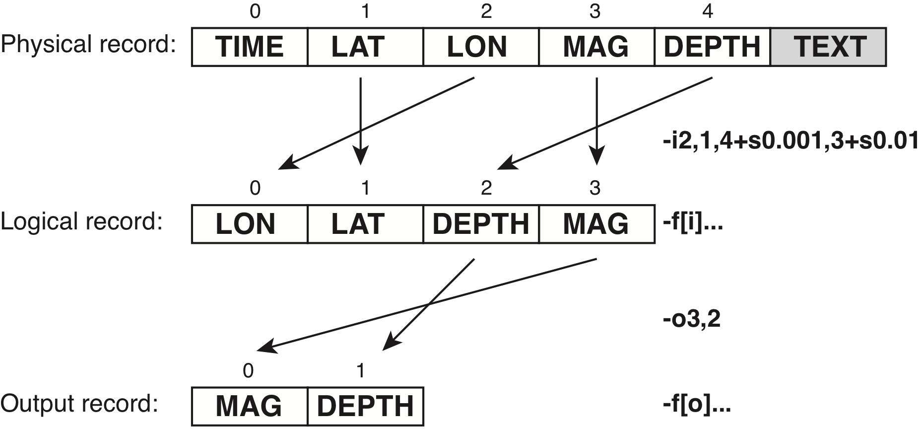
The physical, logical (input) and output record in GMT. Here, we are
reading a file with 5 numerical columns plus some free-form text at the
end. Our module (here plot) will be used to plot circles at the
given locations but we want to assign color based on the depth column
(which we need to convert from meters to km) and symbol size based on the
mag column (but we want to scale the magnitude by 0.01 to get suitable symbol sizes).
We use -i to pull in the desired columns in the required order and apply
the scaling, resulting in a logical input record with 4 columns. The -f option
can be used to specify column types in the logical record if it is not clear
from the data themselves (such as when reading a binary file). Finally, if
a module needs to write out only a portion of the current logical record then
you may use the corresponding -o option to select desired columns, including
the trailing text column t. If you only want to output one word from the
trailing text, then append the word number (0 is the first word). Note that
these column numbers now refer to the logical record, not the physical, since
after reading the data there is no physical record, only the logical record in memory.
4.16. Spherical distance calculations: The -j option
Syntax
- -je|f|g
Determine how spherical distances are calculated in modules that support this [Default is -jg].
Description
GMT has different ways to compute distances on planetary bodies:
-jg to perform great circle distance calculations, with parameters such as distance increments or radii compared against calculated great circle distances [Default is -jg].
-jf to select Flat Earth mode, which gives a more approximate but faster result.
-je to select ellipsoidal (or geodesic) mode for the highest precision and slowest calculation time.
Note: All spherical distance calculations depend on the current ellipsoid (PROJ_ELLIPSOID), the definition of the mean radius (PROJ_MEAN_RADIUS), and the specification of latitude type (PROJ_AUX_LATITUDE). Geodesic distance calculations is also controlled by method (PROJ_GEODESIC).
4.17. Setting automatic legend entries: The -l option
Syntax
-l[label][+Dpen][+Ggap][+Hheader][+L[code/]text][+Ncols][+Ssize[/height]][+V[pen]][+ffont][+gfill][+jjustify][+ooff][+ppen][+sscale][+wwidth]
Add a map legend entry to the session legend information file for the current plot.
Description
The -l option is used to automatically build the specfile that is read by the legend module to create map or plot legends. This allows detailed and complicated legends that mix a variety of items, such as symbols, free text, colorbars, scales, images, and more. Yet, a simple legend will suffice for the vast majority of plots displaying symbols or lines. Optionally, append a text label to describe the entry. The following modifiers are supported to allow further changes to the legend that is built by legend (upper-case modifiers reflect legend codes described in legend, which provides more details and customization):
+D to draw a horizontal line in the given pen before the legend entry is placed [default is no line].
+G to add the vertical space specified by gap [default is no extra space].
+H to add the specified legend header [default is no header].
+L to set a line text. Optionally, prepend a horizontal justification code L(eft), C(enter), or R(ight) for text [default is C].
+N to change the number of columns used to set the following legend items to cols [default is 1].
+S to override the size of the current symbol for the legend or set a height if plotting a line or contour [default uses the same symbol as plotted].
+V to start and +vpen to stop drawing vertical line from previous to current horizontal line [default is no vertical line].
+f to set the font used for the legend header [default is FONT_TITLE].
+g to set the fill used for the legend frame [default is white].
+j to set placement of the legend using the two-character justification code justify [default is TR].
+o to set the offset from legend frame to anchor point [default is 0.2c].
+p to set the pen used for the legend frame [default is 1p].
+s to resize all symbol and length sizes in the legend by scale [default is no scaling].
+w to set legend frame width [default is auto].
Note: Default pen is given by MAP_DEFAULT_PEN. Note: +H, +g, +j, +o, +p, +w, and +s will only take effect if appended to the very first -l option for a plot. The +N modifier, if appended to the first -l option, affects the legend width (unless set via +w); otherwise it just subdivides the available width among the specified columns. If legend is not called explicitly we will call it implicitly when finishing the plot via end. Note: If auto-coloring is used for pens or fills and -l is set then label may contain a C-format for integers (e.g., %3.3d) or just # and we will use the sequence number with the format to build the label entries. Alternatively, give a list of comma-separated labels, or give no label if your segment headers contain label settings. Note: Due to this mechanism, if your single label actually contains commas, you must replace these with the octal code for a comma (\054).
Examples
A simple plot with two symbols can obtain a legend by using this option and modifiers and is shown in Figure Auto Legend:
gmt begin GMT_autolegend
	gmt set GMT_THEME cookbook
	gmt plot -R0/7.2/3/7.2 -Jx2c @Table_5_11.txt -Sc0.35c -Glightgreen -Wfaint -lApples+H"LEGEND"+f16p+D
	gmt plot @Table_5_11.txt -St0.35c -Gorange -B -BWStr -lOranges
	gmt legend -DjTR+w3c+o0.25c -F+p1p+ggray95+s
gmt end show
As the script shows, when no specfile is given to legend then we look for the automatically generated one in the session directory.
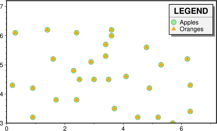
Each of the two plot commands use -l to add a symbol to the auto legend; the first also sets a legend header of given size and draws a horizontal line.
4.18. Grid interpolation parameters: The -n option
Syntax
- -n[b|c|l|n][+a][+bg|p|n][+c][+tthreshold]
Select grid interpolation mode.
Description
The -n option controls parameters used for 2-D grids resampling [default is bicubic interpolation with antialiasing and a threshold of 0.5, using geographic (if grid is known to be geographic) or natural boundary conditions]. Append one of the following to select the type of spline used:
b to use B-spline smoothing.
c to use bicubic interpolation.
l to use bilinear interpolation.
n to use nearest-neighbor value (for example to plot categorical data).
The following modifiers are supported:
+a to switch off antialiasing (where supported) [default uses antialiasing].
+b to override boundary conditions used, by appending g for geographic, p for periodic, or n for natural boundary conditions. For the latter two you may append x or y to specify just one direction, otherwise both are assumed.
+c to clip the interpolated grid to input z-min/z-max [default may exceed limits].
+t to control how close to nodes with NaNs the interpolation will go based on threshold. A threshold of 1.0 requires all (4 or 16) nodes involved in interpolation to be non-NaN. For example, 0.5 will interpolate about half way from a non-NaN value and 0.1 will go about 90% of the way [default is 0.5].
4.19. Output columns selection: The -o option
Syntax
- -ocols[,…][,t[word]]
Select specific data columns for primary output, in arbitrary order.
Description
The -o option allows you to specify which output file physical data columns to use and in what order. Specify individual columns or column ranges in the format start[:inc]:stop, where inc defaults to 1 if not specified, separated by commas [Default writes all columns in order, starting with the first column (i.e., column 0)]. Columns can be repeated. The chosen data columns will be used as given and columns not listed will be skipped. To write from a given column until the end of the record, leave off stop when specifying the column range.
Normally, any trailing text in the internal records will be included in the output, but when -o is used to specify specific columns you must explicitly append the extra “column” t to include the trailing text on output. To only select a single word from the trailing text, append the word number (first word is 0). Finally, -on will simply write the numerical output only and skip any trailing text, while -ot will only output the trailing text (or selected word). Note: If -i is also used then columns given to -o correspond to the order after the -i selection has taken place and not the columns in the original record.
Examples
To write out just the 4th and 2nd data column to the output, use -o3,1 (since 0 is the first column). To write the 4th, 2nd, and 4th again use -o3,1,3.
4.20. Perspective view: The -p option
Syntax
- -p[x|y|z]azim[/elev[/zlevel]][+wlon0/lat0[/z0]][+vx0/y0]
Select perspective view and set the azimuth and elevation of the viewpoint.
Description
All plotting programs that normally produce a flat, two-dimensional illustration can be told to view this flat illustration from a particular vantage point, resulting in a perspective view. You can select perspective view with the -p option by setting the azimuth (azim) of the viewpoint [Default is 180]. The following modifiers are supported:
x|y|z to plot against the “wall” x = level (using x) or y = level (using y) or the horizontal plain (using z) [default is z].
/elev to set the elevation of the viewport [Default is 90].
/zlevel to indicate the z-level at which all 2D material, like the plot frame, is plotted (only valid when -p is used in consort with -Jz or -JZ) [Default is at the bottom of the z-axis].
For frames used for animation, we fix the center of your data domain. Specify another center using one of the following modifiers:
+w to project lon0/lat0 (and z0 if applicable) to the center of the page size.
+v to specify the coordinates of the projected 2-D view point as x0/y0.
When -p is used without any further arguments, the values from the last use of -p in a previous GMT command will be used (in modern mode this also supplies the previous -Jz or -JZ if doing a 3-D region). Alternatively, you can perform a simple rotation about the z-axis by just giving the rotation angle. Optionally, use +v or +w to select another axis location than the plot origin.
4.21. Data row selection: The -q option
Syntax
- -q[i|o][~]rows|limits[+ccol][+a|t|s]
Select specific data rows to be read and/or written.
Description
The -q option is used to select specific data rows to be read (using -q or -qi) or written (using -qo) [Default is all rows]. Specify individual rows or row ranges in the format start[:inc]:stop, where inc defaults to 1 if not specified, separated by commas [Default reads and writes all rows in order, starting with the first row (i.e., row 0)]. To read (or write) from a given row until the end of the data, leave off stop. To select all the rows not specified by the given ranges, prepend the selected rows with a leading ~. Append one of the following modifiers to control how the rows are counted [Default is +a]:
+a to count all rows in the data set.
+t to reset the count at the start of each table.
+s to reset the count at the start of each segment.
Alternatively, use +ccol to indicate that the arguments instead are min/max data limits for the values in column col. With +ccol, only rows whose data for the given column col are within the range(s) given by the min/max limits are read (with -qi) or written (with -qo). Note: Because arguments may contain colons or be negative, you must specify min/max instead of start[:inc]:stop. If min or max is not given we default to -infinity and + infinity, respectively (e.g., -qo50/+c2 will only write records whose z-values (in 3rd column) is ≥ 50 while -qo/50+c2 will only write records whose z-values is ≤ 50).
Note: Header records do not increase the row counters; only data records do.
Examples
Use -q1+s to only read the 2nd data record from each of the segments found.
4.22. Grid registration: The -r option
Syntax
- -r[g|p]
Select gridline or pixel node registration.
Description
All 2-D grids in GMT have their nodes organized in one of two ways, known as gridline and pixel registration. The GMT default is gridline registration (-rg); programs that allow for the creation of grids can use the -r option (or -rp) to select pixel registration instead.
Most observed data tend to be in gridline registration while processed data sometime may be distributed in pixel registration. While you may convert between the two registrations this conversion looses the Nyquist frequency and dampens the other high frequencies. It is best to avoid any registration conversion if you can help it. Planning ahead may be important.
4.22.1. Gridline registration
In this registration, the nodes are centered on the grid line intersections and the data points represent the average value in a cell of dimensions (\(x_{inc} \cdot y_{inc}\)) centered on each node (left side of Figure Grid registration). In the case of grid line registration the number of nodes are related to region and grid spacing by
which for the example in left side of Figure Grid registration yields nx = ny = 4.
4.22.2. Pixel registration
Here, the nodes are centered in the grid cells, i.e., the areas between grid lines, and the data points represent the average values within each cell (right side of Figure Grid registration). In the case of pixel registration the number of nodes are related to region and grid spacing by
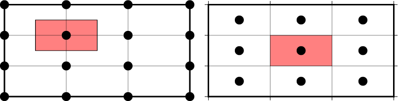
Gridline- and pixel-registration of data nodes. The red shade indicates the areas represented by the value at the node (solid circle).
Here is the source script for the figure above:
gmt begin GMT_registration
gmt set GMT_THEME cookbook
gmt plot -R0/3/0/3 -JX2.5i/1.25i -B1g1 -Bwesn -Wthinner -L -Glightred << EOF
0.5	1.5
1.5	1.5
1.5	2.5
0.5	2.5
EOF
gmt grdmath -R0/3/0/3 -I1 0 = tt.nc
gmt grd2xyz tt.nc | gmt plot -Sc0.12i -N -G0

gmt plot -B1g1 -Bwesn -W0p -L -Glightred -X2.75i << EOF
1	1
2	1
2	2
1	2
EOF
gmt grdmath -R0/3/0/3 -I1 -r 0 = tt.nc
gmt grd2xyz tt.nc | gmt plot -Sc0.12i -Gblack
rm tt.nc
gmt end show
Thus, given the same region (-R) and grid spacing, the pixel-registered grids have one less column and one less row than the gridline-registered grids; here we find nx = ny = 3.
4.22.3. Switching registrations
GMT offer ways to convert a pixel-registered grid to a gridline-registered grid. One way is to simply adjust the region of the grid by half the grid-spacing and toggle the registration in grdedit -T. This is a non-destructive way to convert the grid, but it does change the domain which may not be desirable depending on application. The other is to resample the grid at the other set of nodes via grdsample -T. This approach leaves the region exactly the same but is destructive due to the loss of the higher data frequencies, as shown in Figure Registration resampling.
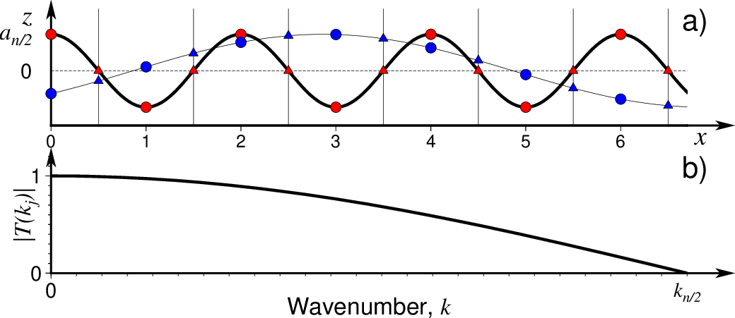
a) Cross-section of a grid along the x-axis for a constant value of y, showing just the Nyquist x-component (heavy line) at its grid nodes (red circles). Resampling this component half-way between nodes (vertical lines) will always give zero (red triangles), hence this signal is lost, unlike long wavelength components (thin line), which can be interpolated (blue triangles). Intermediate wavelengths will experience attenuated amplitudes as well. b) Transfer function for resampling data from a pixel-registered to a gridline-registered grid format illustrates the loss of amplitude that will occur. There is also a linear change in phase from 0 to 90 degrees as a function of wavenumber \(k_j\) [Marks and Smith, 2007 [14].
Here is the source script for the figure above:
gmt begin GMT_grid2pix
	gmt set GMT_THEME cookbook
	gmt subplot begin 2x1 -F6i/2.5i -M3p -A+jTR+o-0.2i/0
		gmt subplot set 0
		gmt math -T0/7/0.02 T PI MUL COS = | gmt plot -R0/6.7/-1.5/1.7 -W2p -Bx1 -By0g10 -BWS --MAP_FRAME_TYPE=graph --MAP_GRID_PEN_PRIMARY=0.25p,-
		gmt basemap -Bx0g1+0.5 -By0 -BS
		gmt math -T0/7/0.02 T PI MUL 4 DIV 2.25 SUB COS = | gmt plot -W0.25p
		gmt math -T0/6/1 T PI MUL COS = | gmt plot -Sc0.1i -Gred -W0.25p -N
		gmt math -T0.5/6.5/1 T 0 MUL = | gmt plot -St0.1i -Gred -W0.25p -N
		gmt math -T0/6/1 T PI MUL 4 DIV 2.25 SUB COS = | gmt plot -Sc0.1i -Gblue -W0.25p -N
		gmt math -T0.5/6.5/1 T PI MUL 4 DIV 2.25 SUB COS = | gmt plot -St0.1i -Gblue -W0.25p -N
		gmt text -N -F+f+j <<- EOF
		6.9 -1.7 18p,Times-Italic RT x
		-0.2 1.6 18p,Times-Italic RT z
		-0.2 1.0 16p,Times-Italic RM a@-n/2@-
		-0.2 0.0 14p,Helvetica RM 0
		EOF
		gmt subplot set 1
		gmt set PS_SCALE_X 0.6 PS_SCALE_Y 0.6 FONT_ANNOT_PRIMARY 14p FONT_LABEL 16p MAP_LABEL_OFFSET 0
		gmt math -T0/0.5/0.001 T PI MUL COS = | gmt plot -R0/0.5/0/1.2 -W2p -Bx1f+l"Wavenumber, @%6%k@%%" -By1f+l"|@%6%T(k@-j@-)@%%|" -BWS --MAP_FRAME_TYPE=graph --MAP_GRID_PEN_PRIMARY=0.25p,-
		gmt text -N -F+f+j <<- EOF
		0.5 -0.1 14p,Times-Italic TC k@-n/2@-
		EOF
	gmt subplot end
gmt end show
4.23. NaN-record treatment: The -s option
Syntax
- -s[cols][+a][+r]
Suppress output of data records whose z-value(s) equal NaN.
Description
The -s option can be used to suppress output for records whose z-value equals NaN [default outputs all records]. Optionally, supply a comma-separated list of all columns or column ranges to consider for this NaN test [default only considers the third data column (i.e., cols = 2)]. Column ranges must be given in the format start[:inc]:stop, where inc defaults to 1 if not specified. The following modifiers are supported:
+r to reverse the suppression, i.e., only output the records whose z-value equals NaN.
+a to suppress the output of the record if just one or more of the columns equal NaN [default skips record only if values in all specified cols equal NaN]
4.24. Layer transparency: The -t option
Syntax
- -ttransp[/transp2][+f|s]
Set transparency level(s) for an overlay.
Description
The -t option allows you to change the transparency level for the current overlay by appending the transp percentage in the 0-100 range [default is 0 (i.e., opaque)]. Normally, transp applies to both fill and stroke, but you can limit the transparency to one of them by appending +f or +s for fill or stroke, respectively. Alternatively, append /transp2 to set separate transparencies for fills and strokes.
Transparency may also be controlled on a feature by feature basis when setting color or fill (see the cookbook section Specifying area fill attributes). Note: The modules plot, plot3d, and text can all change transparency on a record-by-record basis if -t is given without argument and the input file supplies variable transparencies as the last numerical column value(s). Note: The transparency is only visible when PDF or raster format output is selected because the PostScript language does not support transparency. Only the PNG format selection adds a transparency layer in the image (for further processing).
4.25. Examining data cycles: The -w option
Syntax
- -wy|a|w|d|h|m|s|cperiod[/phase][+ccol]
Convert input records to a cyclical coordinate.
Description
The -w option converts the input x-coordinate to a cyclical coordinate, or a different input column if selected via the +c modifier. Temporal data (i.e., regular time series) can be analyzed for periods via standard spectral analysis, such as offered by spectrum1d and grdfft. However, it is often of interest to examine aspects of such periodicities in the time domain. To enable such analyses we need to convert our monotonically increasing time coordinates to periodic or cyclic coordinates so that data from many cycles can be stacked, binned, displayed in histograms, etc. The conversion from input x, y, or z coordinates to wrapped, periodic coordinates follows the simple equation
where t is the input coordinate, \(\tau\) is a phase-shift [Default is zero], and T is the desired period for the modulus operator, yielding cyclic coordinates \(t'\). GMT offers many standard time cycles in prescribed units plus a custom cycle for other types of Cartesian coordinates. The table below shows the values for units, phase and period that are prescribed and only requires the user to specify the corresponding wrapping code (y|a|w|d|h|m|s|cperiod[/phase]):
Code |
Purpose (unit) |
Period |
Phase |
Range |
|---|---|---|---|---|
y |
Yearly cycle (normalized) |
1 year |
0 |
0–1 |
a |
Annual cycle (month) |
1 year |
0 |
0–12 |
w |
Weekly cycle (day) |
1 week |
0 |
0–7 |
d |
Daily cycle (hour) |
1 day |
0 |
0–24 |
h |
Hourly cycle (minute) |
1 hour |
0 |
0–60 |
m |
Minute cycle (second) |
1 minute |
0 |
0–60 |
s |
Second cycle (second) |
1 second |
0 |
0–1 |
c |
Custom cycle (normalized) |
\(T\) |
\(\tau\) |
0–1 |
Optionally, append +ccol to select the input column with the coordinates to be wrapped, [default col is 0, i.e., the first column]. If the custom cycle c is chosen then you must also supply the period and optionally any phase [default is 0] in the same units of your data (i.e., no units should be appended to -w).
Note: Coordinates for w in the range 0-1 correspond to the first day of the week [Monday] but can be changed via TIME_WEEK_START. Note: If a temporal cycle is indicated then we implicitly set -f to indicate absolute time (unless already set separately).
Examples
To demonstrate the use of -w we will make a few plots of the daily discharge rate of the Mississippi river during the 1930-1940 period. A simple time series plot is created by
gmt begin GMT_cycle_1
	gmt set GMT_THEME cookbook
	gmt plot @mississippi.txt -JX15cT/7c -Bxaf -Byaf+l"10@+3@+ m@+3@+/s" -BWSrt+t"Mississippi river daily discharge" -W0.25p,red -i0,1+s1e-3
gmt end show
which results in the plot in Figure Mississippi discharge:
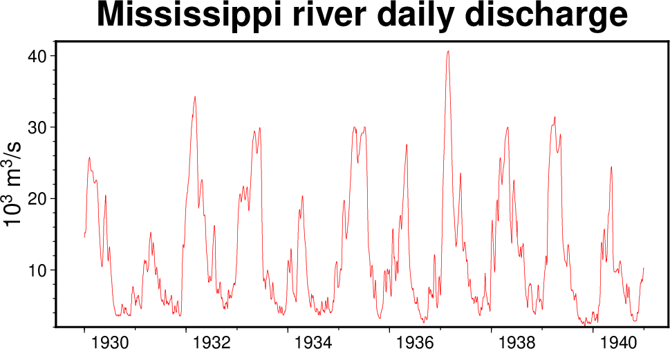
Regular time-series plot of the daily Mississippi river discharge.
Given the clear annual signal we wish to plot this data using a normalized yearly coordinate so that all the years are plotted on top of a single normalized year. We accomplish this feature via -wy and use the prescribed 0–1 year range.
gmt begin GMT_cycle_2
	gmt set GMT_THEME cookbook
	gmt plot @mississippi.txt -R0/1/0/50 -JX15c/7c -W0.25p,red -Bxaf -Byaf+l"10@+3@+ m@+3@+/s" -BWSrt+t"Mississippi river annual discharge" -i0,1+s1e-3 -wy
gmt end show
These commands result in Figure Mississippi annual discharge
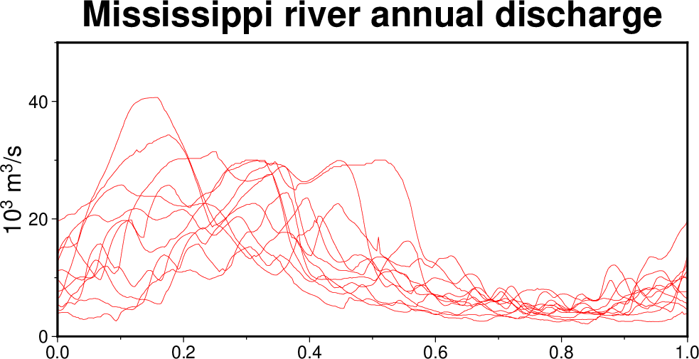
Daily Mississippi river discharge data plotted over the duration of a single, normalized year.
In this representation, both regular and leap years are normalized by their respective lengths. If we prefer to examine the discharge variation as a function of calendar month, then we want all the values belonging to a particular month to fall into the same bin, even though the bins represent variable ranges (28-31 days). For such analyses we are better off using -wa which normalizes the data per month, then adds the integer month number. In other words, all timestamps in March of any year are converted by taking the time since the start of March normalized by the length of March, and then add 2. Thus, all March data from any year will result in coordinates 2.00000–2.999999….. This allows us to easily make a histogram of monthly discharge shown in Figure Mississippi monthly discharge.
gmt begin GMT_cycle_3
	gmt set GMT_THEME cookbook
	gmt histogram @mississippi.txt -R-3/9/0/8 -JX15c/7c -T1 -Gred -W1p -Bxaf -Byaf+l"10@+6@+ m@+3@+/s" -BWSrt+t"Average monthly discharge" -Z0+w -i0,1+s1e-6 -wa
gmt end show
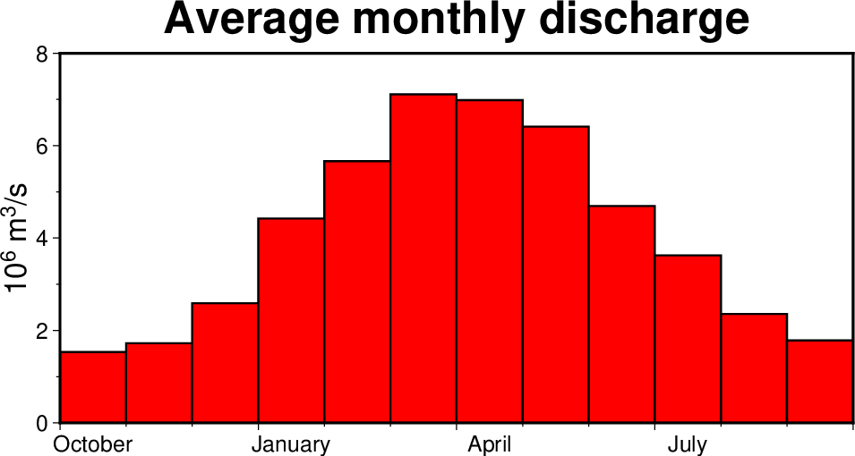
Monthly Mississippi river discharge for the 10-year period, from September to September.
Quarterly discharge would similarly be obtained by using -T3 in the histogram command. As can be seen in Figure Mississippi monthly discharge, the annual cycle axis (as well as a weekly cycle axis) is considered a temporal axis and hence the settings related to the appearance of month and weekday names, such as GMT_LANGUAGE, FORMAT_TIME_PRIMARY_MAP and TIME_WEEK_START, may be used.
Note that the -w option can also be applied to the y-coordinate instead (or any other coordinate) via the +ccol modifier. Below we demonstrate this using the same Mississippi river data but read it in so that time is the y coordinate. The following script generates a subplot with two illustrations similar to the ones above but (basically) transposed:
gmt begin GMT_cycle_4
	gmt set GMT_THEME cookbook
	gmt subplot begin 1x2 -Fs8c/10c -BWSrt -T"Mississippi river annual discharge" -A+jTR
		gmt plot @mississippi.txt -i1+s1e-3,0 -R0/50/0/1 -W0.25p,blue -Byaf+l"Normalized year" -Bxaf+l"10@+3@+ m@+3@+/s" -wy+c1 -c
		gmt histogram @mississippi.txt -R-3/9/0/8 -T1 -Gblue -W1p -Bxaf -Byaf+l"10@+6@+ m@+3@+/s" -Z0+w -i0,1+s1e-6 -A -wa -c  --FORMAT_TIME_PRIMARY_MAP=a
	gmt subplot end
gmt end show
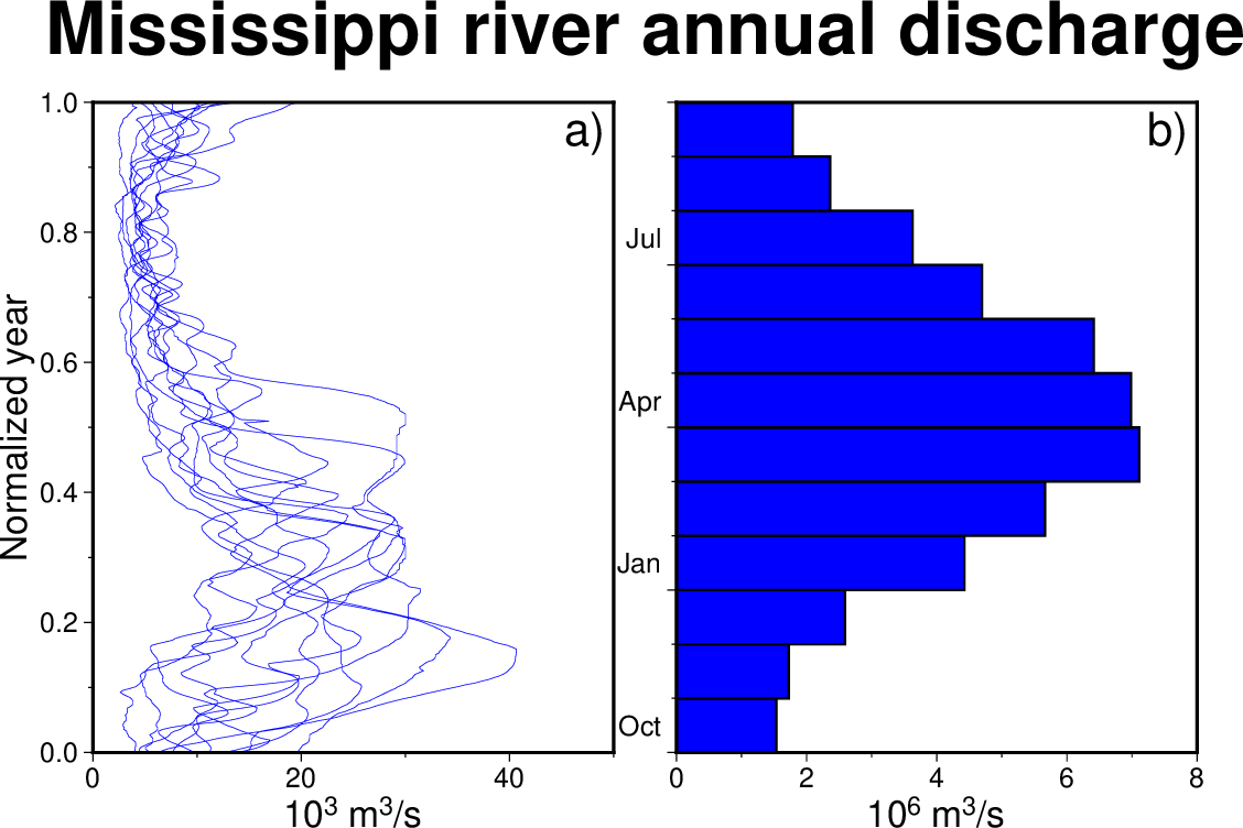
a) Daily Mississippi river discharge data plotted over the duration of a single, normalized year. b) Monthly Mississippi river discharge for the 10-year period, from September to September.
Because -w is a global GMT option it is available in all modules that read tables. Because of this, we can grid the data and make an image of the wrapped dataset:
gmt begin GMT_cycle_5
	gmt set GMT_THEME cookbook
	gmt xyz2grd @mississippi.txt -i0,1+s1e-3,1+s1e-3 -wy -R0/1/0/50 -I50+n -r -Gtmp.grd
 	gmt grdimage tmp.grd -JX15c/8c -BWSen -Bxaf+l"Normalized year" -Byaf+l"Discharge (10@+3@+ m@+3@+/s)"
 	gmt colorbar -DJRM -Baf
gmt end show
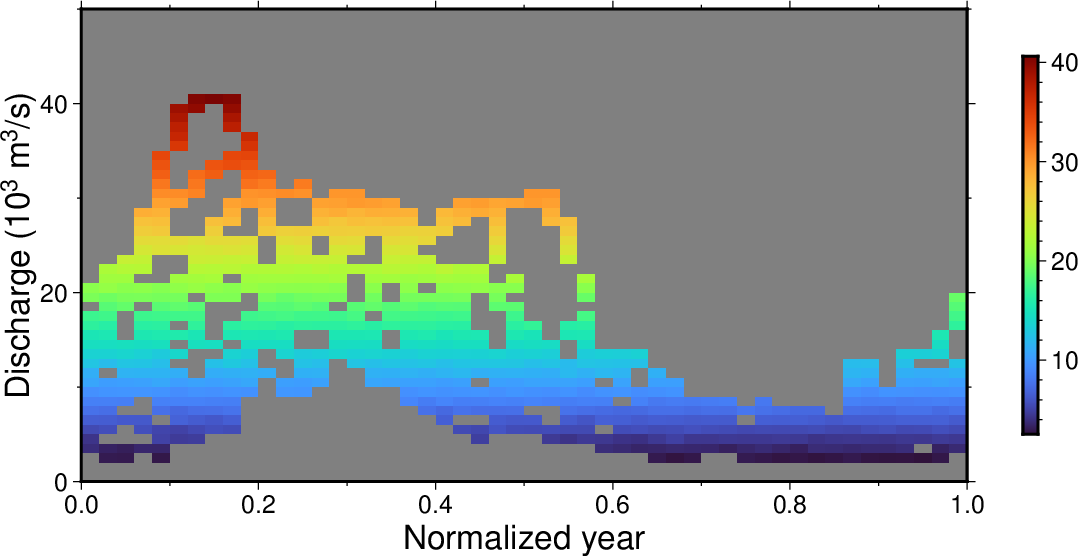
Daily Mississippi river discharge data converted to a grid and imaged with the default (turbo) color table.
Our final example will explore the weekly and daily time-cycles using a three-year data set of traffic (vehicles/hour) crossing the Verrazano-Narrows bridge between Staten Island and Brooklyn (i.e., mostly inbound traffic destined for Manhattan). We will show the raw time-series, wrap it to a weekly period, make a weekly histogram and finally present an hourly histogram. The figure caption under Figure NY traffic discusses the four panels resulting from running the script below:
gmt begin GMT_cycle_6
	gmt set GMT_THEME cookbook
	gmt set TIME_WEEK_START Monday
	gmt subplot begin 2x2 -Fs15c/8c -M14p/6p -A -T"Verrazzano-Narrows Bridge @%34%\337@%% Brooklyn Traffic [2018-2020]" -BWSrt
 		# Raw time-series
		gmt plot @NY_traffic.txt -Wfaint,red -By+l"Vehicles/hour" -gx21600 -c
		# Weekly wrapped time-series
 		gmt plot @NY_traffic.txt -R0/7/0/17000 -Wfaint,red -ww -gx0.25 -c
		# Weekly histogram normalized for number of hours for a weekday in the 3-year data
		n_week_hours=$(gmt convert @NY_traffic.txt -ww | gmt select -Z0/0.999+c0 | gmt info -Fi -o2)
 		gmt histogram @NY_traffic.txt -R0/7/2000/4000 -Wthick -Gred -T1 -Z0+w -By+l"Vehicles/hour" -i0,1+d${n_week_hours} -ww -c
		# Daily histogram normalized for number of days in the 3-year data
		n_mondays=$(gmt convert @NY_traffic.txt -wd | gmt select -Z-0.5/0.5+c0 | gmt info -Fi -o2)
 		gmt histogram @NY_traffic.txt -R0/24/0/8000 -Wthick -Gred -T1 -Z0+w -i0,1+d${n_mondays} -wd -c
 	gmt subplot end
gmt end show
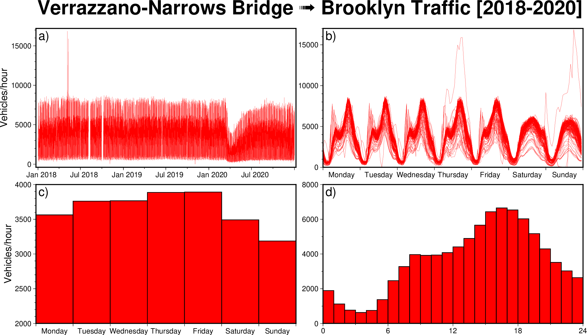
a) Time-series of traffic over a three-year period. Note the dramatic drop as Covid-19 became a major issue in mid-March 2020, as well as some data-gaps and possibly a spike in May 2018. We use -g to skip drawing lines across data gaps exceeding 6 hours. b) Wrapped weekly signals make it easy to see the bimodal morning and evening rush-hour pattern for the weekdays with a different pattern on the weekends (the “spike” in (a) turned out to be data from a single Thursday and Sunday that seem problematic). Again, we use -g to skip data gaps exceeding 6 hours. c) A weekly histogram shows how traffic slowly builds up towards the weekend then drops off towards Sunday. The script calculates the number of repeated hours to normalize the plots. d) A daily histogram is created by wrapping to a daily cycle, then normalizing by the number of days.
4.26. Selecting number of CPU cores: The -x option
Syntax
- -x[[-]n]
Specify the number of active cores to be used in any OpenMP-enabled multi-threaded algorithms.
Description
The -x option limits the number of cores to be used in any OpenMP-enabled multi-threaded algorithms [default is to use all available cores]. Append n to only use n cores (if too large it will be truncated to the maximum cores available). Finally, give a negative n to select (all - n) cores (or at least 1 if n equals or exceeds all). The -x option is only available to GMT modules compiled with OpenMP support, with the exception of movie and batch which handle their own parallel execution.
4.27. Latitude/Longitude or Longitude/Latitude?: The -: option
Syntax
- -:[i|o]
Swap 1st and 2nd column on input and/or output.
Description The -: option swaps the 1st and 2nd column on input and output [default is no swapping]. Append i to select input only or o to select output only [default affects both]. This option is typically used to handle (latitude, longitude) files; see also Input columns selection: The -i option. Note that command line arguments that may take geographic coordinates (e.g., -R) always expect longitude before latitude. Also, geographical grids are expected to have the longitude as first (minor) dimension.