19. Annotation of Contours and “Quoted Lines”

The GMT programs grdcontour (for data given as 2-dimensional grids) and contour (for x,y,z tables) allow for contouring of data sets, while plot and plot3d can plot lines based on x,y- and x,y,z-tables, respectively. In both cases it may be necessary to attach labels to these lines. Clever or optimal placements of labels is a very difficult topic, and GMT provides several algorithms for this placement as well as complete freedom in specifying the attributes of the labels. Because of the richness of these choices we present this Chapter which summarizes the various options and gives several examples of their use.

19.1. Label Placement

GMT provides five different algorithms for determining where labels should be placed. Furthermore, two “symbol” options (-Sq for “quoted line” and -S~ for “decorated line”) in plot and plot3d share these algorithms for text and symbol placements. The contouring programs expect the algorithm to be specified as arguments to -G, while the line plotting programs expect the same arguments to follow -Sq or -S~. The information appended to these options is the same in all three cases and is provided in the form of [code]info. The five algorithms correspond to the five codes below (some codes will appear in both upper and lower case; they share the same algorithm but differ in some other ways). In what follows, the phrase “line segment” is taken to mean either a contour or a line to be labeled or decorated. The codes are:

d:

Full syntax is ddist[c|i|p][/frac]. Place labels according to the distance measured along the projected line on the map. Append the unit you want to measure distances in [Default is taken from PROJ_LENGTH_UNIT]. Starting at the beginning of a line, place labels every dist increment of distance along the line. To ensure that closed lines whose total length is less than dist get annotated, we may append frac which will place the first label at the distance d = dist \(\times\) frac from the start of a closed line (and every dist thereafter). If not given, frac defaults to 0.25.

D:

Full syntax is Ddist[d|m|s|e|f|k|M|n][/frac]. This option is similar to d except the original data must be referred to geographic coordinates (and a map projection must have been chosen) and actual Earth [36] surface distances along the lines are considered. Append the unit you want to measure distances in; choose among arc degree, minute, and second, or meter [Default], feet, kilometer, statute Miles, or nautical miles. Other aspects are similar to code d.

f:

Full syntax is ffix.txt[/slop[c|i|p]]. Here, an ASCII file fix.txt is given which must contain records whose first two columns hold the coordinates of points along the lines at which locations the labels should be placed. Labels will only be placed if the coordinates match the line coordinates to within a distance of slop (append unit or we use PROJ_LENGTH_UNIT). The default slop is zero, meaning only exact coordinate matches will do.

l:

Full syntax is lline1[,line2[, …]]. One or more straight line segments are specified separated by commas, and labels will be placed at the intersections between these lines and our line segments. Each line specification implies a start and stop point, each corresponding to a coordinate pair. These pairs can be regular coordinate pairs (i.e., longitude/latitude separated by a slash), or they can be two-character codes that refer to predetermined points relative to the map region. These codes are taken from the text justification keys [L|C|R][B|M|T] so that the first character determines the x-coordinate and the second determines the y-coordinate. In grdcontour, you can also use the two codes Z+ and Z- as shorthands for the location of the grid’s global maximum and minimum, respectively. For example, the line LT/RB is a diagonal from the upper left to the lower right map corner, while Z-/135W/15S is a line from the grid minimum to the point (135°W, 15°S).

L:

Same as l except we will treat the lines given as great circle start/stop coordinates and fill in the points between before looking for intersections. You must make sure not to give antipodal start and stop coordinates since the great circle path would be undefined.

n:

Full syntax is nnumber[/minlength[c|i|p]]. Place number of labels along each line regardless of total line length. The line is divided into number segments and the labels are placed at the centers of these segments. Optionally, you may give a minlength distance to ensure that no labels are placed closer than this distance to its neighbors.

N:

Full syntax is Nnumber[/minlength[c|i|p]]. Similar to code n but here labels are placed at the ends of each segment (for number >= 2). A special case arises for number = 1 when a single label will be placed according to the sign of number: -1 places one label justified at the start of the line, while +1 places one label justified at the end of the line.

s:

Similar to n but splits input lines into a series of two-point line segments first. The rest of the algorithm them operates on these sets of lines. This code (and S) are specific to quoted and decorated lines.

S:

Similar to N but with the modification described for s.

x:

Full syntax is xcross.txt. Here, an ASCII file cross.txt is a multi-segment file whose lines will intersect our segment lines; labels will be placed at these intersections.

X:

Same as x except we treat the lines given as great circle start/stop coordinates and fill in the points between before looking for intersections.

Only one algorithm can be specified at any given time.

19.2. Label Attributes

Determining where to place labels is half the battle. The other half is to specify exactly what are the attributes of the labels. It turns out that there are quite a few possible attributes that we may want to control, hence understanding how to specify these attributes becomes important. In the contouring programs, one or more attributes may be appended to the -A option using the format +code[args] for each attribute, whereas for the line plotting programs these attributes are appended to the -Sq option following a colon (:) that separates the label codes from the placement algorithm. Several of the attributes do not apply to contours so we start off with listing those that apply universally. These codes are:

+a:

Controls the angle of the label relative to the angle of the line. Append n for normal to the line, give a fixed angle measured counter-clockwise relative to the horizontal. or append p for parallel to the line [Default]. If using grdcontour the latter option you may further append u or d to get annotations whose upper edge always face the next higher or lower contour line.

+c:

Surrounding each label is an imaginary label “textbox” which defines a region in which no segment lines should be visible. The initial box provides an exact fit to the enclosed text but clearance may be extended in both the horizontal and vertical directions (relative to the label baseline) by the given amounts. If these should be different amounts please separate them by a slash; otherwise the single value applies to both directions. Append the distance units of your choice (c|i|m|p), or give % to indicate that the clearance should be this fixed percentage of the label font size in use. The default is 15%.

+d:

Debug mode. This is useful when testing contour placement as it will draw the normally invisible helper lines and points in the label placement algorithms above.

+e:

Delayed mode, to delay the plotting of the text as text clipping is set instead.

+f:

Specifies the desired label font, including size or color. See text for font names or numbers. The default font is given by FONT_ANNOT_PRIMARY.

+g:

Selects opaque rather than the default transparent text boxes. You may optionally append the color you want to fill the label boxes; the default is the same as PS_PAGE_COLOR.

+j:

Selects the justification of the label relative to the placement points determined above. Normally this is center/mid justified (CM in text justification parlance) and this is indeed the default setting. Override by using this option and append another justification key code from [L|C|R][B|M|T]. Note for curved text (+v) only vertical justification will be affected.

+o:

Request a rounded, rectangular label box shape; the default is rectangular. This is only manifested if the box is filled or outlined, neither of which is implied by this option alone (see +g and +p). As this option only applies to straight text, it is ignored if +v is given.

+p:

Selects the drawing of the label box outline; append your preferred pen unless you want the default GMT pen [0.25p,black].

+r:

Do not place labels at points along the line whose local radius of curvature falls below the given threshold value. Append the radius unit of your choice (c|i|p) [Default is 0].

+u:

Append the chosen unit to the label. Normally a space will separate the label and the unit. If you want to close this gap, append a unit that begins with a hyphen (-). If you are contouring with grdcontour and you specify this option without appending a unit, the unit will be taken from the z-unit attribute of the grid header.

+v:

Place curved labels that follow the wiggles of the line segments. This is especially useful if the labels are long relative to the length-scale of the wiggles. The default places labels on an invisible straight line at the angle determined.

+w:

The angle of the line at the point of straight label placement is calculated by a least-squares fit to the width closest points. If not specified, width defaults to 10.

+=:

Similar in most regards to +u but applies instead to a label prefix which you must append.

For contours, the label will be the value of the contour (possibly modified by +u or +=). However, for quoted lines other options apply:

+l:

Append a fixed label that will be placed at all label locations. If the label contains spaces you must place it inside matching quotes.

+L:

Append a code flag that will determine the label. Available codes are:

+Lh:

Take the label from the current multi-segment header (hence it is assumed that the input line segments are given in the multi-segment file format; if not we pick the single label from the file’s header record). We first scan the header for an embedded -Llabel option; if none is found we instead use the first word following the segment marker [>].

+Ld:

Take the Cartesian plot distances along the line as the label; append c|i|p as the unit [Default is PROJ_LENGTH_UNIT]. The label will be formatted according to the FORMAT_FLOAT_OUT string, unless label placement was determined from map distances along the segment lines, in which case we determine the appropriate format from the distance value itself.

+LD:

Calculate actual Earth surface distances and use the distance at the label placement point as the label; append d|e|f|k|m|M|n|s to specify the unit [If not given we default to degrees, unless label placement was determined from map distances along the segment lines, in which case we use the same unit specified for that algorithm]. Requires a map projection to be used.

+Lf:

Use all text after the 2nd column in the fixed label location file fix.txt as labels. This choice obviously requires the fixed label location algorithm (code f) to be in effect.

+Ln:

Use the running number of the current multi-segment as label.

+LN:

Use a slash-separated combination of the current file number and the current multi-segment number as label.

+Lx:

As h but use the multi-segment headers in the cross.txt file instead. This choice obviously requires the crossing segments location algorithm (code x|X) to be in effect.

19.3. Examples of Contour Label Placement

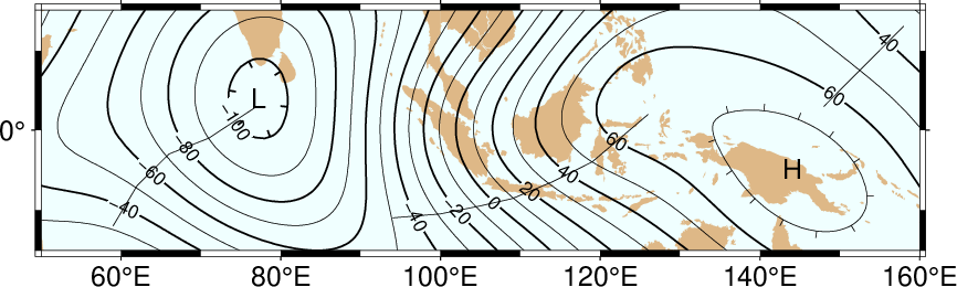
We will demonstrate the use of these options with a few simple examples. First, we will contour a subset of the global geoid data used in Example (1) Contour maps; the region selected encompasses the world’s strongest “geoid dipole”: the Indian Low and the New Guinea High.

19.3.1. Equidistant labels

Our first example uses the default placement algorithm. Because of the size of the map we request contour labels every 1.5 inches along the lines:

gmt begin GMT_App_O_1
	gmt set GMT_THEME cookbook
	gmt coast -R50/160/-15/15 -JM5.3i -Gburlywood -Sazure -A500
	gmt grdcontour @App_O_geoid.nc -B20f10 -BWSne -C10 -A20+f8p -Gd1.5i -S10 -T+lLH
gmt end show

As seen in Figure Contour label 1, the contours are placed rather arbitrary. The string of contours for -40 to 60 align well but that is a fortuitous consequence of reaching the 1.5 inch distance from the start at the bottom of the map.

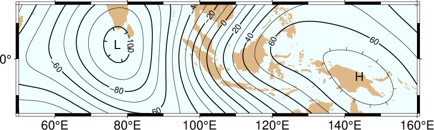
Equidistant contour label placement with -Gd, the only algorithm available in previous GMT versions.

19.3.2. Fixed number of labels

We now exercise the option for specifying exactly how many labels each contour line should have:

gmt begin GMT_App_O_2
	gmt set GMT_THEME cookbook
	gmt coast -R50/160/-15/15 -JM5.3i -Gburlywood -Sazure -A500
	gmt grdcontour @App_O_geoid.nc -B20f10 -BWSne -C10 -A20+f8p -Gn1/1i -S10 -T+lLH
gmt end show

By selecting only one label per contour and requiring that labels only be placed on contour lines whose length exceed 1 inch, we achieve the effect shown in Figure Contour label 2.

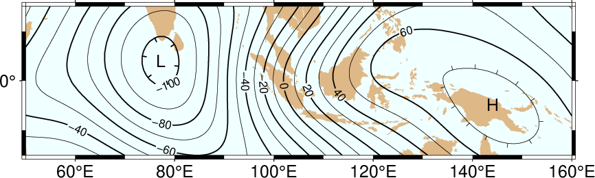
Placing one label per contour that exceed 1 inch in length, centered on the segment with -Gn.

19.3.3. Prescribed label placements

Here, we specify four points where we would like contour labels to be placed. Our points are not exactly on the contour lines so we give a nonzero “slop” to be used in the distance calculations: The point on the contour closest to our fixed points and within the given maximum distance will host the label.

cat << EOF > fix.txt
80      -8.5
55      -7.5
102     0
130     10.5
EOF
gmt begin GMT_App_O_3
	gmt set GMT_THEME cookbook
	gmt coast -R50/160/-15/15 -JM5.3i -Gburlywood -Sazure -A500
	gmt grdcontour @App_O_geoid.nc -B20f10 -BWSne -C10 -A20+d+f8p -Gffix.txt/0.1i -S10 -T+lLH
gmt end show

The angle of the label is evaluated from the contour line geometry, and the final result is shown in Figure Contour label 3. To aid in understanding the algorithm we chose to specify “debug” mode (+d) which placed a small circle at each of the fixed points.

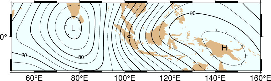
Four labels are positioned on the points along the contours that are closest to the locations given in the file fix.txt in the -Gf option.

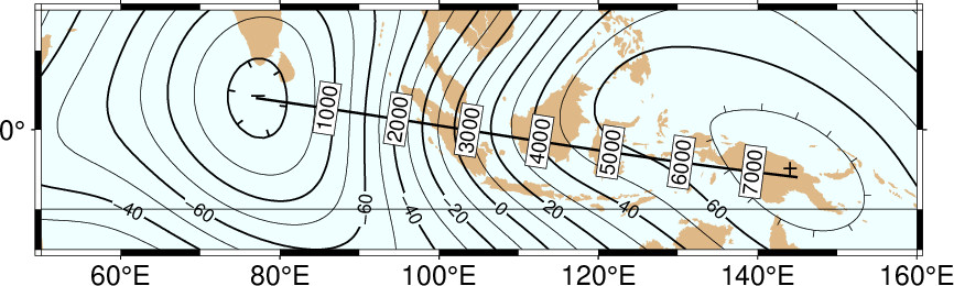
19.3.4. Label placement at simple line intersections

Often, it will suffice to place contours at the imaginary intersections between the contour lines and a well-placed straight line segment. The -Gl or -GL algorithms work well in those cases:

gmt begin GMT_App_O_4
	gmt set GMT_THEME cookbook
	gmt coast -R50/160/-15/15 -JM5.3i -Gburlywood -Sazure -A500
	gmt grdcontour @App_O_geoid.nc -B20f10 -BWSne -C10 -A20+d+f8p -GLZ-/Z+ -S10 -T+lLH
gmt end show

The obvious choice in this example is to specify a great circle between the high and the low, thus placing all labels between these extrema.

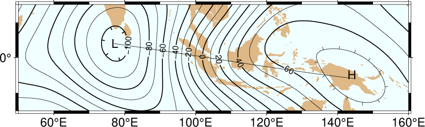
Labels are placed at the intersections between contours and the great circle specified in the -GL option.

The thin debug line in Figure Contour label 4 shows the great circle and the intersections where labels are plotted. Note that any number of such lines could be specified; here we are content with just one.

19.3.5. Label placement at general line intersections

If (1) the number of intersecting straight line segments needed to pick the desired label positions becomes too large to be given conveniently on the command line, or (2) we have another data set or lines whose intersections we wish to use, the general crossing algorithm makes more sense:

gmt begin GMT_App_O_5
	gmt set GMT_THEME cookbook
	gmt coast -R50/160/-15/15 -JM5.3i -Gburlywood -Sazure -A500
	gmt grdcontour @App_O_geoid.nc -B20f10 -BWSne -C10 -A20+d+f8p -GX@App_O_cross.txt -S10 -T+lLH
gmt end show

Labels are placed at the intersections between contours and the multi-segment lines specified in the -GX option.

In this case, we have created three strands of lines whose intersections with the contours define the label placements, presented in Figure Contour label 5.

19.4. Examples of Label Attributes

We will now demonstrate some of the ways to play with the label attributes. To do so we will use plot on a great-circle line connecting the geoid extrema, along which we have sampled the ETOPO5 relief data set. The file thus contains lon, lat, dist, geoid, relief, with distances in km.

19.4.1. Label placement by along-track distances, 1

This example will change the orientation of labels from along-track to across-track, and surrounds the labels with an opaque, outlined text box so that the label is more readable. We choose the place the labels every 1000 km along the line and use that distance as the label. The labels are placed normal to the line:

gmt begin GMT_App_O_6
	gmt set GMT_THEME cookbook
	gmt coast -R50/160/-15/15 -JM5.3i -Gburlywood -Sazure -A500
	gmt grdcontour @App_O_geoid.nc -B20f10 -BWSne -C10 -A20+d+f8p -Gl50/10S/160/10S -S10 -T+l
	gmt plot -SqD1000k:+g+LD+an+p -Wthick @App_O_transect.txt
gmt end show

Labels attributes are controlled with the arguments to the -Sq option.

The composite illustration in Figure Contour label 6 shows the new effects. Note that the line connecting the extrema does not end exactly at the ‘-’ and ‘+’ symbols. This is because the placements of those symbols are based on the mean coordinates of the contour and not the locations of the (local or global) extrema.

19.4.2. Label placement by along-track distances, 2

A small variation on this theme is to place the labels parallel to the line, use spherical degrees for placement, append the degree symbol as a unit for the labels, choose a rounded rectangular text box, and inverse-video the label:

gmt begin GMT_App_O_7
	gmt set GMT_THEME cookbook
	gmt coast -R50/160/-15/15 -JM5.3i -Gburlywood -Sazure -A500
	gmt grdcontour @App_O_geoid.nc -B20f10 -BWSne -C10 -A20+d+u" m"+f8p -Gl50/10S/160/10S -S10 -T+l
	gmt plot -SqD15d:+gblack+fwhite+Ld+o+u@. -Wthick @App_O_transect.txt
gmt end show

The output is presented as Figure Contour label 7.

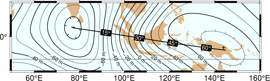
Another label attribute example.

19.4.3. Using a different data set for labels

In the next example we will use the bathymetry values along the transect as our label, with placement determined by the distance along track. We choose to place labels every 1500 km. To do this we need to pull out those records whose distances are multiples of 1500 km and create a “fixed points” file that can be used to place labels and specify the labels. This is done with awk.

gmt begin GMT_App_O_8
	gmt set GMT_THEME cookbook
	gmt convert -i0,1,4 -Em150 @App_O_transect.txt | $AWK '{print $1,$2,int($3)}' > fix2.txt
	gmt coast -R50/160/-15/15 -JM5.3i -Gburlywood -Sazure -A500
	gmt grdcontour @App_O_geoid.nc -B20f10 -BWSne -C10 -A20+d+u" m"+f8p -Gl50/10S/160/10S -S10 -T+l
	gmt plot -Sqffix2.txt:+g+an+p+Lf+u" m"+f8p -Wthick @App_O_transect.txt
gmt end show

The output is presented as Figure Contour label 8.

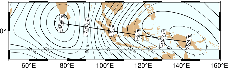
Labels based on another data set (here bathymetry) while the placement is based on distances.

19.5. Putting it all together

Finally, we will make a more complex composite illustration that uses several of the label placement and label attribute settings discussed in the previous sections. We make a map showing the tsunami travel times (in hours) from a hypothetical catastrophic landslide in the Canary Islands [37]. We lay down a color map based on the travel times and the shape of the seafloor, and travel time contours with curved labels as well as a few quoted lines. The final script is

gmt begin GMT_App_O_9
gmt set GMT_THEME cookbook
R=-R-85/5/10/55
gmt grdgradient @earth_relief_05m_g $R -Nt1 -A45 -Gtopo5_int.nc
gmt set FORMAT_GEO_MAP ddd:mm:ssF FONT_ANNOT_PRIMARY +9p FONT_TITLE 22p
gmt project -E-74/41 -C-17/28 -G10 -Q > great_NY_Canaries.txt
gmt project -E-74/41 -C2.33/48.87 -G100 -Q > great_NY_Paris.txt
km=$(echo -17 28 | gmt mapproject -G-74/41+uk -fg --FORMAT_FLOAT_OUT=%.0f -o2)
gmt makecpt -Clightred,lightyellow,lightgreen -T0,3,6,100 -N
gmt grdimage @App_O_ttt.nc -Itopo5_int.nc -C $R -JM5.3i -nc+t1
gmt grdcontour @App_O_ttt.nc -C0.5 -A1+u" hour"+v+f8p,Bookman-Demi \
	-GL80W/31N/17W/26N,17W/28N/17W/50N -S2
gmt plot -Wfatter,white great_NY_Canaries.txt
gmt coast -B20f5 -BWSne+t"Tsunami travel times from the Canaries" -N1/thick \
	-Glightgray -Wfaint -A500
gmt convert great_NY_*.txt -E | gmt plot $R -Sa0.15i -Gred -Wthin
gmt plot -Wthick great_NY_Canaries.txt \
	-Sqn1:+f8p,Times-Italic+l"Distance Canaries to New York = $km km"+ap+v
gmt plot great_NY_Paris.txt -Sc0.08c -Gblack
gmt plot -Wthinner great_NY_Paris.txt -SqD1000k:+an+o+gblue+LDk+f7p,Helvetica-Bold,white
cat << EOF | gmt text -Gwhite -Wthin -Dj0.1i -F+f8p,Bookman-Demi+j
74W	41N	RT	New York
2.33E	48.87N	CT	Paris
17W	28N	CT	Canaries
EOF
gmt end show

with the complete illustration presented as Figure Contour label 9.

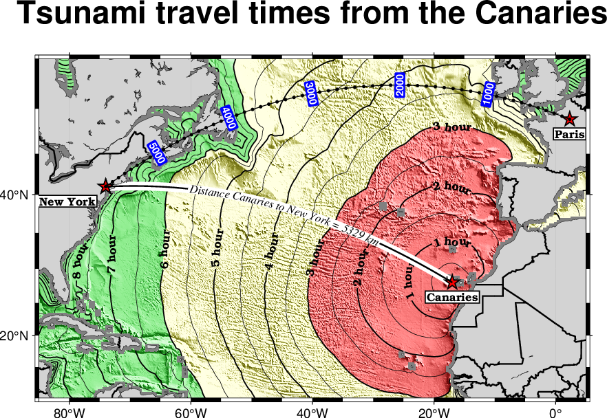
Tsunami travel times from the Canary Islands to places in the Atlantic, in particular New York. Should a catastrophic landslide occur it is possible that New York will experience a large tsunami about 8 hours after the event.

19.6. Footnotes

[36]

or whatever planet we are dealing with.

[37]

Travel times were calculated using Geoware’s travel time calculator, ttt; see http://www.geoware-online.com/.