plot
Plot lines, polygons, and symbols in 2-D
Synopsis
gmt plot [ table ] -Jparameters -Rwest/east/south/north[/zmin/zmax][+r][+uunit] [ -A[m|p|x|y|r|t] ] [ -B[p|s]parameters ] [ -Ccpt ] [ -Ddx/dy ] [ -E[x|y|X|Y][+a|A][+cl|f][+n][+wcap][+ppen] ] [ -F[c|n|r][a|f|s|r|refpoint] ] [ -Gfill|+z ] [ -H[scale] ] [ -I[intens] ] [ -L[+b|d|D][+xl|r|x0][+yb|t|y0][+ppen] ] [ -N[c|r] ] [ -S[symbol][size] ] [ -T ] [ -U[stamp] ] [ -V[level] ] [ -W[pen][attr] ] [ -X[a|c|f|r][xshift] ] [ -Y[a|c|f|r][yshift] ] [ -Zvalue|file] [ -aflags ] [ -bibinary ] [ -dinodata[+ccol] ] [ -eregexp ] [ -fflags ] [ -ggaps ] [ -hheaders ] [ -iflags ] [ -lflags ] [ -pflags ] [ -qiflags ] [ -ttransp ] [ -wflags ] [ -:[i|o] ] [ --PAR=value ]
Description
Reads (x,y) pairs from files [or standard input] and will plot lines, polygons, or symbols at those locations on a map. If a symbol is selected and no symbol size given, then it will interpret the third column of the input data as symbol size. Symbols whose size is <= 0 are skipped. If no symbols are specified then the symbol code (see -S below) must be present as last column in the input. If -S is not used, a line connecting the data points will be drawn instead. To explicitly close polygons, use -L. Select a fill with -G. If -G is set, -W will control whether the polygon outline is drawn or not. If a symbol is selected, -G and -W determines the fill and outline/no outline, respectively.
Required Arguments
- table
One or more ASCII (or binary, see -bi[ncols][type]) data table file(s) holding a number of data columns. If no tables are given then we read from standard input.
- -Jparameters
Specify the projection. (See full description) (See cookbook summary) (See projections table).
- -Rxmin/xmax/ymin/ymax[+r][+uunit]
Specify the region of interest. Note: If using modern mode and -R is not provided, the region will be set based on previous plotting commands. If this is the first plotting command in the modern mode levels and -R is not provided, the region will be automatically determined based on the data in table (equivalent to using -Ra). (See full description) (See cookbook information).
For perspective view -p, optionally append /zmin/zmax. (more …)
Optional Arguments
- -A[m|p|x|y|r|t]
By default, geographic line segments are drawn as great circle arcs by resampling coarse input data along such arcs. To disable this sampling and draw them as straight lines, use the -A flag. Alternatively, add m to draw the line by first following a meridian, then a parallel. Or append p to start following a parallel, then a meridian. (This can be practical to draw a line along parallels, for example). For Cartesian data, points are simply connected, unless you append x or y to draw stair-case curves that whose first move is along x or y, respectively. For polar projection, append r or t to draw stair-case curves that whose first move is along r or theta, respectively.
- -B[p|s]parameters
Set map boundary frame and axes attributes. (See full description) (See cookbook information).
- -Ccpt
Give a CPT or specify -Ccolor1,color2[,color3,…] to build a linear continuous CPT from those colors automatically, where z starts at 0 and is incremented by one for each color. In this case colorn can be a r/g/b triplet, a color name, or an HTML hexadecimal color (e.g. #aabbcc ). If -S is set, let symbol fill color be determined by the z-value in the third column. Additional fields are shifted over by one column (optional size would be 4th rather than 3rd field, etc.). If -S is not set, then it expects the user to supply a multisegment file where each segment header contains a -Zvalue string. The value will control the color of the line or polygon (if -L is set) via the CPT. Alternatively, see the -Z option for how to assign z-values. Note: If modern mode and no argument is given then we select the current CPT.
- -Ddx/dy
Offset the plot symbol or line locations by the given amounts dx/dy [Default is no offset]. If dy is not given it is set equal to dx. You may append dimensional units from c|i|p to each value.
- -E[x|y|X|Y][+a|A][+cl|f][+n][+wcap][+ppen]
Draw symmetrical error bars. Append x and/or y to indicate which bars you want to draw (Default is both x and y). The x and/or y errors must be stored in the columns after the (x,y) pair [or (x,y,z) triplet]. If +a is appended then we will draw asymmetrical error bars; these requires two rather than one extra data column, with the two signed deviations. Use +A to read the low and high bounds rather than signed deviations. If upper case X and/or Y are used we will instead draw “box-and-whisker” (or “stem-and-leaf”) symbols. The x (or y) coordinate is then taken as the median value, and four more columns are expected to contain the minimum (0% quantile), the 25% quantile, the 75% quantile, and the maximum (100% quantile) values. The 25-75% box may be filled by using -G. If +n is appended the we draw a notched “box-and-whisker” symbol where the notch width reflects the uncertainty in the median. This symbol requires a 5th extra data column to contain the number of points in the distribution. The +w modifier sets the cap width that indicates the length of the end-cap on the error bars [7p]. Pen attributes for error bars may also be set via +ppen. [Defaults: width = default, color = black, style = solid]. When -C is used we can control how the look-up color is applied to our symbol. Append +cf to use it to fill the symbol, while +cl will just set the error pen color and turn off symbol fill. Giving +c will set both color items. Note: The error bars are placed behind symbols except for the large vertical and horizontal bar symbols (-Sb|B) where they are plotted on top to avoid the lower bounds being obscured.
- -F[c|n|p][a|f|s|r|refpoint]
Alter the way points are connected (by specifying a scheme) and data are grouped (by specifying a method). Append one of three line connection schemes: c: Draw continuous line segments for each group [Default]. p: Draw line segments from a reference point reset for each group. n: Draw networks of line segments between all points in each group. Optionally, append the one of four segmentation methods to define the group: a: Ignore all segment headers, i.e., let all points belong to a single group, and set group reference point to the very first point of the first file. f: Consider all data in each file to be a single separate group and reset the group reference point to the first point of each group. s: Segment headers are honored so each segment is a group; the group reference point is reset to the first point of each incoming segment [Default]. r: Same as s, but the group reference point is reset after each record to the previous point (this method is only available with the -Fp scheme). Instead of the codes a|f|s|r you may append the coordinates of a refpoint which will serve as a fixed external reference point for all groups.
- -Gfill|+z (more …)
Select color or pattern for filling of symbols or polygons [Default is no fill]. Note that this module will search for -G and -W strings in all the segment headers and let any values thus found over-ride the command line settings. If -Z is set, use -G+z to assign fill color via -Ccpt and the z-values obtained. Finally, if fill = auto[-segment] or auto-table then we will cycle through the fill colors implied by COLOR_SET and change on a per-segment or per-table basis. Any transparency setting is unchanged.
- -H[scale]
Scale symbol sizes and pen widths on a per-record basis using the scale read from the data set, given as the first column after the (optional) z and size columns [no scaling]. The symbol size is either provided by -S or via the input size column. Alternatively, append a constant scale that should be used instead of reading a scale column.
- -Iintens
Use the supplied intens value (nominally in the -1 to +1 range) to modulate the fill color by simulating illumination [none]. If no intensity is provided we will instead read intens from the first data column after the symbol parameters (if given).
- -L[+b|d|D][+xl|r|x0][+yb|t|y0][+ppen] Example
X
-L example
cat << EOF > t.txt 1 1 2 3 3 2 4 4 EOF gmt begin filler pdf gmt plot -R0/5/0/5 -JX3i -B t.txt -Gred -W2p -L+yb gmt plot -B t.txt -Gred -W2p -L+yt -X3.25i gmt plot -B t.txt -Gred -W2p -L+xl -X-3.25i -Y3.25i gmt plot -B t.txt -Gred -W2p -L+xr -X3.25i gmt plot -B t.txt -Gred -W2p -L+y4 -X-3.25i -Y3.25i gmt plot -B t.txt -Gred -W2p -L+x4.5 -X3.25i gmt end show
Force closed polygons. Alternatively, append modifiers to build a polygon from a line segment. Append +d to build symmetrical envelope around y(x) using deviations dy(x) given in extra column 3. Append +D to build asymmetrical envelope around y(x) using deviations dy1(x) and dy2(x) from extra columns 3-4. Append +b to build asymmetrical envelope around y(x) using bounds yl(x) and yh(x) from extra columns 3-4. Append +xl|r|x0 to connect first and last point to anchor points at either xmin, xmax, or x0, or append +yb|t|y0 to connect first and last point to anchor points at either ymin, ymax, or y0. Polygon may be painted (-G) and optionally outlined by adding +ppen [no outline]. Note: When option -Z is passed via segment headers you will need -L to ensure your segments are interpreted as polygons, else they are seen as lines.
- -N[c|r]
Do NOT clip symbols that fall outside map border [Default plots points whose coordinates are strictly inside the map border only]. The option does not apply to lines and polygons which are always clipped to the map region. For periodic (360-longitude) maps we must plot all symbols twice in case they are clipped by the repeating boundary. The -N will turn off clipping and not plot repeating symbols. Use -Nr to turn off clipping but retain the plotting of such repeating symbols, or use -Nc to retain clipping but turn off plotting of repeating symbols.
- -S[symbol][size]
Plot symbols (including vectors, wedges, fronts, decorated or quoted lines). If present, size is symbol size in the default unit set by PROJ_LENGTH_UNIT (unless c, i, or p is appended). If the symbol code (see below) is not given it will be read from the last column in the input data; this scheme cannot be used in conjunction with binary input. Optionally, append c, i, or p to indicate that the size information in the input data is in units of cm, inch, or point, respectively [Default is PROJ_LENGTH_UNIT]. Note: If you provide both size and symbol via the input file you must use PROJ_LENGTH_UNIT to indicate the unit used for the symbol size or append the units to the sizes listed in the file. If symbol sizes are expected via one or more data columns then you may convert those values to suitable symbol sizes via the -i mechanism. The general input expectations are:
coordinates [ value ] [ parameters ] [ symbol ]
where coordinates is two or three columns specifying the location of a point, the optional value is required when -C is used to control color, the optional parameters is required when no symbol size is specified, and the trailing text with leading symbol code is required when the symbol code is not specified on the command line. Note: parameters may represent more than one size column as some symbols require several parameters to be defined (e.g., a circle just needs one column, a rectangle needs two dimensions, while an ellipse needs an orientation and two dimensions, and so on); see specifics below. When there is only a single parameter we will refer to it as size.
You can also change symbols by adding the required -S option to any of your multi-segment headers.
We will first outline the 14 basic geometric symbols that only require a single parameter: size.
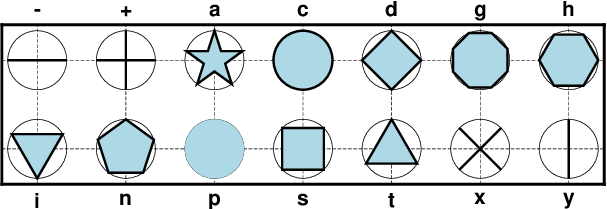
The 14 basic geometric symbols available, shown with their symbol codes. Four symbols (-|+|x|y) are line-symbols only (-W), one (the point p only takes a color via -G) while the rest may have outline (-W) and fill (-G) specified. The thin circles represent the circumscribing circle of the same size.
- -S-size
x-dash (-). size is the length of a short horizontal (x-dir) line segment.
- -S+size
Plus (+). size is diameter of circumscribing circle.
- -Sasize
Star. size is diameter of circumscribing circle.
- -Scsize
circle. size is diameter of circle.
- -Sdsize
diamond. size is diameter of circumscribing circle.
- -Sgsize
Octagon. size is diameter of circumscribing circle.
- -Shsize
hexagon. size is diameter of circumscribing circle.
- -Sisize
inverted triangle. size is diameter of circumscribing circle.
- -Snsize
Pentagon. size is diameter of circumscribing circle.
- -Spsize
point. No size needs to be specified (1 pixel is used).
- -Sssize
square. size is diameter of circumscribing circle.
- -Stsize
triangle. size is diameter of circumscribing circle.
- -Sxsize
Cross (x). size is diameter of circumscribing circle.
- -Sysize
y-dash (|). size is the length of a short vertical (y-dir) line segment.
Note: The uppercase symbols A, C, D, G, H, I, N, S, T are normalized to have the same area as a circle with diameter size, while the size of the corresponding lowercase symbols refers to the diameter of a circumscribed circle.
The next collection shows five symbols that require two or more parameters, and some have optional modifiers to enhance the symbol appearance.
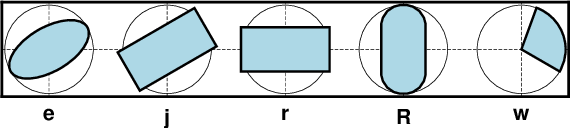
Five basic geometric multi-parameter symbols, shown with their symbol codes. All take two or three parameters to define the symbol; see below for details. Upper-case versions E, J, and W are similar to e, j and w but expect geographic azimuths and distances.
- -Sedirection/major_axis/minor_axis
ellipse. If not given, then direction (in degrees counter-clockwise from horizontal), major_axis, and minor_axis must be found after the coordinates [and value] columns. This option yields a Cartesian ellipse whose shape is unaffected by the map projection. If only a single size is given then we plot a degenerate ellipse (circle) with given diameter.
- -SEazimuth/major_axis/minor_axis
Same as -Se, except azimuth (in degrees east of north) should be given instead of direction. The azimuth will be mapped into an angle based on the chosen map projection (-Se leaves the directions unchanged.) Furthermore, major_axis and minor_axis must be given in geographical instead of plot-distance units. For degenerate ellipses (i.e., circles) with just a diameter given via the input data, use -SE-. For a linear projection we assume the dimensions are given in the same units as -R. For allowable geographical units, see Units and append desired unit to the dimension(s); if dimensions are read from the input then either just append the unit for these values or append the unit to each dimension in the file (do not do both) [Default is k for km]. The shape of the ellipse will be affected by the properties of the map projection.
- -Sjdirection/width/height
Rotated rectangle. If not given, then direction (in degrees counter-clockwise from horizontal), width, and height must be found after the location [and value] columns. If only a single size is given then we plot a degenerate rectangle (square) with given size.
- -SJazimuth/width/height
Same as -Sj, except azimuth (in degrees east of north) should be given instead of direction. The azimuth will be mapped into an angle based on the chosen map projection (-Sj leaves the directions unchanged.) Furthermore, the two dimensions must be given in geographical instead of plot-distance units. For a degenerate rectangle (i.e., square) with one dimension expected to be given via the input data, use -SJ-. For a linear projection we assume the dimensions are given in the same units as -R. For allowable geographical units, see Units and append desired unit to the dimension(s); if dimensions are read from the input then either just append the unit for these values or append the unit to each dimension in the file (do not do both) [Default is k for km]. The shape of the rectangle will be affected by the properties of the map projection.
- -Srwidth/height
rectangle. If width/height are not given, then these dimensions must be found after the location [and value] columns. Alternatively, append +s and then the diagonal corner coordinates are expected after the location [and value] columns instead.
- -SRwidth/height/radius
Rounded rectangle. If width/height/radius are not given, then the two dimensions and corner radius must be found after the location [and value] columns.
- -Sw[outer[/startdir/stopdir]][+i[inner]]
Pie wedge. Give the outer diameter outer, startdir and stopdir. These are directions (in degrees counter-clockwise from horizontal) for wedge. Parameters not appended are read from file after the location [and value] columns. Append +i and append a nonzero inner diameter inner or it will be read last [0]. Append +a[dr] to draw the arc line (at inner and outer diameter); if dr is appended then we draw all arc lines separated radially by dr. Append +r[da] to draw radial lines (at start and stop directions) if da is appended then we draw all radial lines separated angularly by da. These spider-web lines are drawn using the current pen unless +ppen is added.
- -SW[outer[/startaz/stopaz]][+i[inner]]
Same as -Sw, except azimuths (in degrees east of north) should be given instead of the two directions. The azimuths will be mapped into angles based on the chosen map projection (-Sw leaves the directions unchanged). The two diameters are expected in geographic units. For allowable geographical units, see Units and append desired unit to the dimension(s); if dimensions are read from the input then either just append the unit for these values or append the unit to each dimension in the file (do not do both) [Default is k for km]. However, if specified on the command line we also accept plot dimension units. Append +i and append a nonzero inner diameter inner or it will be read last [0]. Append +a[dr] to draw the arc line (at inner and outer diameter); if dr is appended then we draw all arc lines separated radially by dr. Append +r[da] to draw radial lines (at start and stop directions) if da is appended then we draw all radial lines separated angularly by da. These spider-web lines are drawn using the current pen unless +ppen is added.
Text is normally placed with text but there are times we wish to treat a character of even a string as a symbol to be plotted:
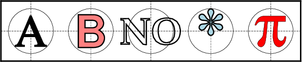
A text symbol can be any letter or string (up to 256 characters) and you may specify specific fonts (size and type) and control outline and the fill properties. Note there is no mechanism to perfectly center the string; see -D to make a simple global adjustment.
- -Slsize+tstring[+a|Aangle][+ffont][+jjustify]
letter or text string (less than 256 characters). Give size, and append +tstring after the size. Note: The size is only approximate; no individual scaling is done for different characters. Remember to escape special characters like *. Optionally, you may append +a to change the angle with the horiontal [0] or use +A to indicate map azimuth instead, +ffont to select a particular font [Default is FONT_ANNOT_PRIMARY] and +jjustify to change justification [CM].
The next type of symbol is the horizontal or vertical bar:
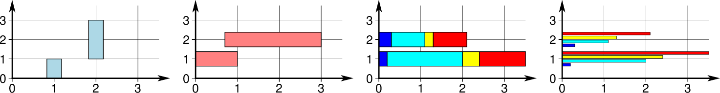
We may place vertical (b) or horizontal (B) bars, and they may extend from the base of your choosing. The thickness of a bar can be a given dimension or can be specified in the units of that axis so its width scales with the projection and region. Using modifiers +v or +i you can also plot multi-band bars with colors set via -C, and +s can represent those as groups of individual bars instead.
- -Sb[size[c|i|p|q]][+b|B[base]][+v|iny][+s[gap]]
Vertical bar extending from base to y. The size is bar width. Append q if size is a quantity in x-units [Default is plot-distance units]. By default, base = 0. Append +b[base] to change this value. If base is not appended then we read it from the last input data column. Use +B[base] if the bar height is measured relative to base [Relative to origin]. Normally, the bar requires a single input y-value. To plot multi-band bars, please append +v|iny, where ny indicates the total number of bands in the bar. Here, +i means we must accumulate the bar values from the increments dy, while +v means we get the complete values relative to base. Normally, the bands are plotted as sections of a final single bar. Use +s to instead split the bar into ny side-by-side, individual and thinner bars. The optional gap is a percent (of fraction) of size for adding gaps between the bars [none], where size is the combined width of all the individual, thinner bars plus the gaps. Multiband bars requires -C with one color per band (CPT z-values must be 0, 1, …, ny - 1). Thus, input records are either (x y1 y2 … yn) or (x dy1 dy2 … dyn).
- -SB[size[c|i|p|q]][+b|B[base]][+v|inx][+s[gap]]
Horizontal bar extending from base to x. The size is bar width. Append q if size is a quantity in y-units [Default is plot-distance units]. By default, base = 0. Append +b[base] to change this value. If base is not appended then we read it from the last input data column. Use +B[base] if the bar length is measured relative to base [Relative to origin]. Normally, the bar requires a single input x-value. To plot multi-band bars, please append +v|inx, where nx indicates the total number of bands in the bar. Here, +i means we must accumulate the bar value from the increments dx, while +v means we get the complete values relative to base. Normally, the bands are plotted as sections of a final single bar. Use +s to instead split the bar into nx side-by-side, individual and thinner bars. The optional gap is a percent (of fraction) of size for adding gaps between the bars [none], where size is the combined width of all the individual, thinner bars plus the gaps. Multiband bars requires -C with one color per band (CPT z-values must be 0, 1, …, nx - 1). Thus, input records are either (x1 y x2 … xn) or (dx1 y dx2 … dxn).
The next family of symbols are all different types of vectors. Apart from requiring parameters such as length and direction (or optionally the coordinates of the end point), we also offer a rich set of modifiers to customize the vector head(s).
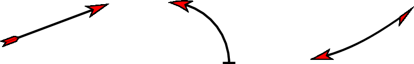
There are three classes of vectors: Cartesian (left), circular (center) and geographic (right). While their use is slightly different, they all share common modifiers that affect how they are displayed.
- -Smsize[+vecmodifiers]
math angle arc, optionally with one or two arrow heads [Default is no arrow heads]. The size is the length of the vector head. Arc width is set by -W, with vector head outlines defaulting to half of arc width. The radius of the arc and its start and stop directions (in degrees counter-clockwise from horizontal) must be given after the location [and value] columns. See Vector Attributes for specifying other attributes.
- -SMsize[+vecmodifiers]
Same as -Sm but switches to straight angle symbol if start and stop angles subtend 90 degrees exactly.
- -Svsize[+vecmodifiers]
vector. The direction (in degrees counter-clockwise from horizontal) and length must be found after the location [and value] columns, and size, if not specified on the command-line, should be present as well, pushing the other items to later columns. The size is the length of the vector head. Vector stem width is set by -W, with head outline pen width defaulting to half of stem pen width. See Vector Attributes for specifying this and other attributes.
- -SVsize[+vecmodifiers]
Same as -Sv, except azimuth (in degrees east of north) should be given instead of direction. The azimuth will be mapped into an angle based on the chosen map projection (-Sv leaves the directions unchanged.) If your length is not in plot units but in arbitrary user units (e.g., a rate in mm/yr) then you can use the -i option to scale the corresponding column via the +sscale modifier. See Vector Attributes for specifying symbol attributes.
- -S=size[+vecmodifiers]
Geographic vector. Here, azimuth (in degrees east from north) and geographical length must be found after the location [and value] columns. The size is the length of the vector head. Vector width is set by -W. See Vector Attributes for specifying attributes. Note: Geovector stems are drawn as thin filled polygons and hence pen attributes like dashed and dotted are not available. For allowable geographical units for the length, see Units [k]. If your length is not in distance units but in arbitrary user units (e.g., a rate in mm/yr) then you can use the -i option to scale the corresponding column via the +sscale modifier.
The next symbol is the programmable custom symbol:
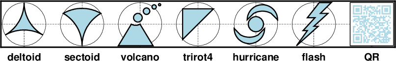
Custom symbols are designed using the Custom Symbol Macro Language. We supply about 40 custom symbols, and users have contributed discipline-specific symbols for structural geology and marine biology that you can explore from the RESOURCES page, so you have lots of examples to use as a template. The language allows you to design symbols that take many parameters and can make decisions based on these parameters.
- -Skname/size
kustom symbol. We will look for a symbol definition file called name.def in (1) the current directory, (2) in ~/.gmt or (3) in $GMT_SHAREDIR/custom. The symbol defined in the definition file is of normalized unit size by default; the appended size will scale the symbol accordingly. Users may create their own custom *.def files; see Custom Symbols below. Alternatively, you can supply an EPS file instead of a *.def file and we will scale and place that graphic as a symbol.
The last group of symbols are all special lines with embellishments along them. The first symbol is called a front and has specific symbols distributed along the curve. Typical uses are weather fronts, fault lines, and more. While the line appearance is controlled by -W, there are many modifiers to control the selection and appearance of the along-line symbols:
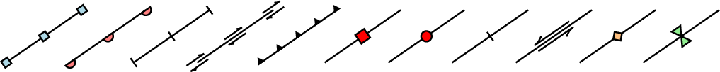
Fronts offer various symbols, such as squares, triangles and circles that may be plotted centered or as a half-symbols on one side. Special options exist for indicating motion (e.g., faults) along a line.
- -Sf[±]gap[/size][+l|+r][+b|c|f|s[angle]|t|v][+ooffset][+p[pen]].
Draw a front. Supply distance gap between symbols and symbol size. If gap is negative, it is interpreted to mean the number of symbols along the front instead. If gap has a leading + then we use the value exactly as given [Default will start and end each line with a symbol, hence the gap is adjusted to fit]. If size is missing it is set to 30% of the gap, except when gap is negative and size is thus required. Append +l or +r to plot symbols on the left or right side of the front [Default is centered]. Append +type to specify which symbol to plot: box, circle, fault, slip, triangle or inverted triangle. [Default is fault]. Slip means left-lateral or right-lateral strike-slip arrows (centered is not an option). The +s modifier optionally accepts the angle used to draw the vector [20]. Alternatively, use +S which draws arcuate arrow heads. Append +ooffset to offset the first symbol from the beginning of the front by that amount [0]. The chosen symbol is drawn with the same pen as set for the line (i.e., via -W). To use an alternate pen, append +ppen. To skip the outline, just use +p with no argument. To make the main front line invisible, add +i. Note: By placing -Sf options in the segment headers that differ from the one on the command line you can change the front types on a segment-by-segment basis.
The next type of embellished line is called a quoted line, which is our term for a line with text along it, similar to an annotated contour in a contour map. There is a rich set of directives and modifiers available to select a specific outcome:

Quoted lines (-Sq) are lines with text. However, the text can be static, read via files, or be quantities computed along the line. This example just shows a wiggly line with a text-aligned label. A rich set of modifier controls the appearance.
- -Sqd|D|f|l|L|n|N|s|S|x|Xposinfo[:labelinfo]
quoted line, i.e., lines with occasional annotations such as contours. Append a required algorithm code and posinfo that control the placement of labels along the quoted lines. Note: The colon separates the algorithm settings from the label information. Choose among six controlling algorithms:
- ddist[c|i|p][/frac] or Ddist[d|e|f|k|m|M|n|s][/frac]
For lower case d, give distances between labels on the plot in your preferred measurement unit c (cm), i (inch), or p (points), while for upper case D, specify distances in map units and append the unit; choose among e (m), f (foot), k (km), M (mile), n (nautical mile) or u (US survey foot), and d (arc degree), m (arc minute), or s (arc second). [Default is 10c or 4i]. As an option, you can append append frac which will place the first label at the distance d = dist \(\times\) frac from the start of a line (and every dist thereafter). If not given, frac defaults to 0.25.
- ffile.txt[/slop[c|i|p]]
Read the ASCII file file.txt and places labels at locations in the file that best matches locations along the quoted lines. Labels will only be placed if the coordinates match the line coordinates to within a distance of slop (append desired unit or we use PROJ_LENGTH_UNIT). The default slop is zero, meaning only exact coordinate matches will do.
- l|Lline1[,line2,…]
Give the coordinates of the end points for one or more comma-separated straight line segments. Labels will be placed where these lines intersect the quoted lines. The format of each line specification is start_lon/start_lat/stop_lon/stop_lat. Both start_lon/start_lat and stop_lon/stop_lat can be replaced by a 2-character key that uses the justification format employed in text to indicate a point on the frame or center of the map, given as [LCR][BMT]. Alternatively, select L to interpret the point pairs as defining great circle segments [Default is straight lines].
- n|Nn_label[/min_dist[c|i|p]]
Specify the number of equidistant labels for quoted lines [1]. Upper case N starts labeling exactly at the start of the line [Default centers them along the line]. N-1 places one justified label at start, while N+1 places one justified label at the end of quoted lines. Optionally, append /min_dist[c|i|p] to enforce a minimum distance separation between successive labels.
- s|Sn_label[/min_dist[c|i|p]]
Same as n|Nn_label but implies that the input data are first to be converted into a series of 2-point line segments before plotting.
- x|Xxfile.txt
Read the ASCII multisegment file xfile.txt and places labels at the intersections between the quoted lines and the lines in xfile.txt. X will resample the lines first along great-circle arcs. In addition, you may optionally append +rradius[c|i|p] to set a minimum label separation in the x-y plane [no limitation].
The optional labelinfo controls the specifics of the label formatting. If not provided we default to the text “N/A”. The argument consists of a concatenated string made up of any of the following modifiers:
- +aangle
Force annotations at a fixed angle, +an for line-normal, or +ap for line-parallel [Default].
- +cdx[/dy]
Set clearance between label and optional text box. Append c|i|p to specify the unit or % to indicate a percentage of the label font size [15%].
- +d[pen]
Turn on debug, which will draw helper points and lines to illustrate the workings of the quoted line setup. Optionally append the pen to use [MAP_DEFAULT_PEN].
- +e
Delay plotting of the text. This is used to build a clip path based on the text, then lay down other overlays while that clip path is in effect, then turning off clipping with clip -Cs which finally plots the pending text.
- +ffont
Set the desired font [Default FONT_ANNOT_PRIMARY with its size changed to 9p].
- +g[color]
Select opaque text boxes [Default is transparent]; optionally specify the color [Default is PS_PAGE_COLOR].
- +i
Make the main quoted line invisible [Draw it per -W].
- +jjust
Set label justification [Default is MC]. Ignored when -SqN|n+|-1 is used.
- +llabel
Set the constant label text. Note: if the text length exceeds the line length then no text will appear.
- +Lflag
Set the label text according to the specified flag:
+Lh Take the label from the current segment header (first scan for an embedded -Llabel option, if not use the first word following the segment flag). For multiple-word labels, enclose entire label in double quotes. +Ld Take the Cartesian plot distances along the line as the label; append c|i|p as the unit [Default is PROJ_LENGTH_UNIT]. +LD Calculate actual map distances; append d|e|f|k|n|M|n|s as the unit [Default is d(egrees), unless label placement was based on map distances along the lines in which case we use the same unit specified for that algorithm]. Requires a map projection to be used. +Lf Use text after the 2nd column in the fixed label location file as the label. Requires the fixed label location setting. +Lx As +Lh but use the headers in the xfile.txt instead. Requires the crossing file option.
- +ndx[/dy]
Nudge the placement of labels by the specified amount (append c|i|p to specify the units). Increments are considered in the coordinate system defined by the orientation of the line; use +N to force increments in the plot x/y coordinates system [no nudging]. Not allowed with +v.
- +o
Select rounded rectangular text box [Default is rectangular]. Not applicable for curved text (+v) and only makes sense for opaque text boxes.
- +p[pen]
Draw outline of text boxes [Default is no outline]; optionally specify pen for outline [Default is width = 0.25p, color = black, style = solid].
- +rmin_rad
Will not place labels where the line’s radius of curvature is less than min_rad [Default is 0].
- +t[file]
Save line label x, y, angle, text to file [Line_labels.txt].
- +uunit
Append unit to all line labels [Default is no unit].
- +v
Specify curved labels following the path [Default is straight labels].
- +w
Specify how many (x,y) points will be used to estimate smooth label angles [Default is 10].
- +x[first,last]
Append the suffixes first and last to the corresponding labels. This modifier is only available when -SqN2 is in effect. Used to annotate the start and end of a line (e.g., a cross-section), append two text strings separated by comma [Default just adds a prime to the second label].
- +=prefix
Prepend prefix to all line labels [Default is no prefix].
Note: By placing -Sq options in the segment headers that differ from the one on the command line you can change the quoted text attributes on a segment-by-segment basis.
The final type of embellished line is called a decorated line (-S~). It is a hybrid between a front and quoted lines in that it offers symbols similar to a front but the placement can be specified in ways similar to the quoted line. However, no built-in clipping exists, such as for quoted lines:

Decorated lines with eleven squares evenly spaced along the line. By default, the symbol is aligned with the line trend, but numerous modifiers allow you to customize the appearance, including to make the line invisible.
- -S~d|D|f|l|L|n|N|s|S|x|Xposinfo:symbolinfo
Decorated line, i.e., lines with symbols placed along them. Append a required algorithm code and posinfo that control the placement of symbols along the decorated lines. Note: The colon separates the algorithm settings from the required symbol information. Choose among six controlling algorithms:
- ddist[c|i|p][/frac] or Ddist[d|e|f|k|m|M|n|s][/frac]
For lower case d, give distances between symbols on the plot in your preferred measurement unit c (cm), i (inch), or p (points), while for upper case D, specify distances in map units and append the unit; choose among e (m), f (foot), k (km), M (mile), n (nautical mile) or u (US survey foot), and d (arc degree), m (arc minute), or s (arc second). [Default is 10c or 4i]. As an option, you can append append frac which will place the first symbol at the distance d = dist \(\times\) frac from the start of a line (and every dist thereafter). If not given, frac defaults to 0.25.
- ffile.txt[/slop[c|i|p]]
Read the ASCII file file.txt and place symbols at locations in the file that matches locations along the decorated lines. Symbols will only be placed if the coordinates match the line coordinates to within a distance of slop (append desired unit or we use PROJ_LENGTH_UNIT). The default slop is zero, meaning only exact coordinate matches will do.
- l|Lline1[,line2,…]
Give the coordinates of the end points for one or more comma-separated straight line segments. Symbols will be placed where these lines intersect the decorated lines. The format of each line specification is start_lon/start_lat/stop_lon/stop_lat. Both start_lon/start_lat and stop_lon/stop_lat can be replaced by a 2-character key that uses the justification format employed in text to indicate a point on the frame or center of the map, given as [LCR][BMT]. L will interpret the point pairs as defining great circles [Default is straight line].
- n|Nn_symbol[/min_dist[c|i|p]]
Specify the number of equidistant symbols for decorated lines [1]. Upper case N starts placing symbols exactly at the start of the line [Default centers them along the line]. N-1 places one symbol at start, while N+1 places one symbol at the end of decorated lines. Optionally, append /min_dist[c|i|p] to enforce a minimum distance separation between successive symbols.
- s|Sn_symbol[/min_dist[c|i|p]]
Same as n|Nn_symbol but implies that the input data are first to be converted into a series of 2-point line segments before plotting.
- x|Xxfile.txt
Read the ASCII multisegment file xfile.txt and places symbols at the intersections between the decorated lines and the lines in xfile.txt. X will resample the lines first along great-circle arcs.
The required symbolinfo controls the specifics of the symbol selection and formatting and consists of a concatenated string made up of any of the following modifiers:
- +aangle
Force symbols at a fixed angle, +an for line-normal, or +ap for line-parallel [Default].
- +d[pen]
Turn on debug, which will draw helper points and lines to illustrate the workings of the decorated line setup. Optionally append the pen to use [MAP_DEFAULT_PEN].
- +g[fill]
Set the symbol fill [no fill].
- +i
Make the main decorated line invisible [Draw it using pen settings provided by -W].
- +ndx[/dy]
Nudge the placement of symbols by the specified amount (append c|i|p to specify the units). Increments are considered in the coordinate system defined by the orientation of the line; use +N to force increments in the plot x/y coordinates system [no nudging].
- +p[pen]
Draw the outline of symbols [Default is no outline]; optionally specify pen for outline [Default is width = 0.25p, color = black, style = solid].
- +s<symbol><size> or +skcustomsymbol/size
Specify the code and size of the decorative symbol. Custom symbols need to be simple, i.e., not require data columns, or be a single EPS file. Hence, valid symbols are limited to the plain geometric one-parameter symbols and the custom symbol (k).
- +w
Specify how many (x,y) points will be used to estimate symbol angles [Default is 10].
If neither +g nor +p are set we select the default pen outline (MAP_DEFAULT_PEN). Note: By placing -S~ options in the segment headers that differ from the one on the command line you can change the decorated lines on a segment-by-segment basis.
- -T
Ignore all input files. If -B is not used then -R -J are not required. Typically used to move plot origin via -X and -Y.
- -U[label|+c][+jjust][+odx[/dy]]
Draw GMT time stamp logo on plot. (See full description) (See cookbook information).
- -V[level]
Select verbosity level [w]. (See full description) (See cookbook information).
- -W[pen][attr] (more …)
Set pen attributes for lines or the outline of symbols [Defaults: width = default, color = black, style = solid]. If the modifier +cl is appended then the color of the line are taken from the CPT (see -C). If instead modifier +cf is appended then the color from the cpt file is applied to symbol fill. Use just +c for both effects. You can also append one or more additional line attribute modifiers: +ooffsetunit will start and stop drawing the line the given distance offsets from the end point. Append unit unit from c|i|p to indicate plot distance on the map or append map distance units instead (see below) [Cartesian distances]; +s will draw the line using a Bezier spline [linear spline]; +vvspecs will place a vector head at the ends of the lines. You can use +vb and +ve to specify separate vector specs at each end [shared specs]. Because +v may take additional modifiers it must necessarily be given at the end of the pen specification. See the Vector Attributes for more information. If -Z is set, then append +z to -W to assign pen color via -Ccpt and the z-values obtained. Finally, if pen color = auto[-segment] or auto-table then we will cycle through the pen colors implied by COLOR_SET and change on a per-segment or per-table basis. The width, style, or transparency settings are unchanged.
- -X[a|c|f|r][xshift]
Shift plot origin. (See full description) (See cookbook information).
- -Y[a|c|f|r][yshift]
Shift plot origin. (See full description) (See cookbook information).
- -Zvalue|file
Instead of specifying a symbol or polygon fill and outline color via -G and -W, give both a value via -Z and a color lookup table via -C. Alternatively, give the name of a file with one z-value (read from the last column) for each polygon in the input data. To apply the color obtained to a fill, use -G+z; to apply it to the pen color, append +z to -W.
- -a[[col=]name[,…]] (more …)
Set aspatial column associations col=name.
- -birecord[+b|l] (more …)
Select native binary format for primary table input. [Default is the required number of columns given the chosen settings].
- -dinodata[+ccol] (more …)
Replace input columns that equal nodata with NaN.
- -e[~]“pattern” | -e[~]/regexp/[i] (more …)
Only accept data records that match the given pattern.
- -f[i|o]colinfo (more …)
Specify data types of input and/or output columns.
- -gx|y|z|d|X|Y|Dgap[u][+a][+ccol][+n|p] (more …)
Determine data gaps and line breaks. The -g option is ignored if -S is set.
- -h[i|o][n][+c][+d][+msegheader][+rremark][+ttitle] (more …)
Skip or produce header record(s).
- -icols[+l][+ddivisor][+sscale|d|k][+ooffset][,…][,t[word]] (more …)
Select input columns and transformations (0 is first column, t is trailing text, append word to read one word only).
- -l[label][+Dpen][+Ggap][+Hheader][+L[code/]txt][+Ncols][+Ssize[/height]][+V[pen]][+ffont][+gfill][+jjust][+ooff][+ppen][+sscale][+wwidth] (more …)
Add a legend entry for the symbol or line being plotted.
- -qi[~]rows|limits[+ccol][+a|t|s] (more …)
Select input rows or data limit(s) [default is all rows].
- -:[i|o] (more …)
Swap 1st and 2nd column on input and/or output.
- -p[x|y|z]azim[/elev[/zlevel]][+wlon0/lat0[/z0]][+vx0/y0] (more …)
Select perspective view.
- -t[transp[/transp2]][+f][+s]
Set transparency level for an overlay, in [0-100] percent range. [Default is 0, i.e., opaque]. Only visible when PDF or raster format output is selected. Only the PNG format selection adds a transparency layer in the image (for further processing). If given, transp applies to both fill and stroke, but you can limit the transparency to one of them by appending +f or +s for fill or stroke, respectively. Alternatively, append /transp2 to set separate transparencies for fills and strokes. If no transparencies are given then we expect to read them from the last numerical column(s). Use the modifiers to indicate which one(s) we should be reading (if both are requested, fill transparency is expected before stroke transparency in the column order). If just -t is given then we interpret it to mean -t+f for fill transparency only.
- -wy|a|w|d|h|m|s|cperiod[/phase][+ccol] (more …)
Convert an input coordinate to a cyclical coordinate.
- -^ or just -
Print a short message about the syntax of the command, then exit (Note: on Windows just use -).
- -+ or just +
Print an extensive usage (help) message, including the explanation of any module-specific option (but not the GMT common options), then exit.
- -? or no arguments
Print a complete usage (help) message, including the explanation of all options, then exit.
- --PAR=value
Temporarily override a GMT default setting; repeatable. See gmt.conf for parameters.
Units
For map distance unit, append unit d for arc degree, m for arc minute, and s for arc second, or e for meter [Default unless stated otherwise], f for foot, k for km, M for statute mile, n for nautical mile, and u for US survey foot. By default we compute such distances using a spherical approximation with great circles (-jg) using the authalic radius (see PROJ_MEAN_RADIUS). You can use -jf to perform “Flat Earth” calculations (quicker but less accurate) or -je to perform exact geodesic calculations (slower but more accurate; see PROJ_GEODESIC for method used).
Vector Attributes
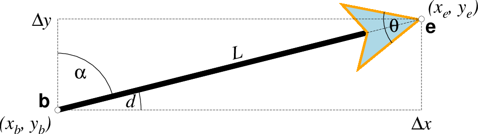
Vector attributes are controlled by options and modifiers. We will refer to this figure and the labels therein when introducing the corresponding modifiers. All vectors require you to specify the begin point \(x_b, y_b\) and the end point \(x_e, y_e\), or alternatively the direction d and length L, while for map projections we usually specify the azimuth \(\alpha\) instead.
Several modifiers may be appended to vector-producing options for specifying the placement of vector heads, their shapes, and the justification of the vector. Below, left and right refers to the side of the vector line when viewed from the beginning point (b) to the end point (e) of a line segment:
+aangle sets the angle \(\theta\) of the vector head apex [30].
+b places a vector head at the beginning of the vector path [none]. Optionally, append t for a terminal line, c for a circle, a for arrow [Default], i for tail, A for plain open arrow, and I for plain open tail. Note: For geovectors only a and A are available. Further append l|r to only draw the left or right half-sides of this head [both sides].
+c selects the vector data quantity magnitude for use with CPT color look-up [Default requires a separate data column following the 2 or 3 coordinates]. Requires that data quantity scaling (with unit q via +v or +z) and a CPT have been selected.
+e places a vector head at the end of the vector path [none]. Optionally, append t for a terminal line, c for a circle, a for arrow [Default], i for tail, A for plain open arrow, and I for plain open tail. Note: For geovectors only a and A are available. Further append l|r to only draw the left or right half-sides of this head [both sides].
+g[fill] sets the vector head fill [Default fill is used, which may be no fill]. Turn off vector head fill by not appending a fill. Some modules have a separate -Gfill option and if used will select the fill as well.
+hshape sets the shape of the vector head (range -2/2). Default is controlled by MAP_VECTOR_SHAPE [default is theme dependent]. A zero value produces no notch. Positive values moves the notch toward the head apex while a negative value moves it away. The example above uses +h0.5.
+m places a vector head at the mid-point the vector path [none]. Append f or r for forward or reverse direction of the vector [forward]. Optionally, append t for a terminal line, c for a circle, a for arrow [Default], i for tail, A for plain open arrow, and I for plain open tail. Further append l|r to only draw the left or right half-sides of this head [both sides]. Cannot be combined with +b or +e.
+n[norm[/min]] scales down vector attributes (pen thickness, head size) with decreasing length, where vector plot lengths shorter than norm will have their attributes scaled by length/norm [other arrow attributes remain invariant to length]. Optionally, append /min for the minimum shrink factor (in the 0-1 range) that we will shrink to [0.25]. For Cartesian vectors, please specify a norm in plot units, while for geovectors specify a norm in map units (see Distance units) [k]. Alternatively, append unit q to indicate we should use user quantity units in making the decision; this means the user also must select user quantity input via +v or +z.
If no argument is given then +n ensures vector heads are not shrunk and always plotted regardless of vector length [Vector heads are not plotted if exceeding vector length].
+o[plon/plat] specifies the oblique pole for the great or small circles. Only needed for great circles if +q is given. If no pole is appended then we default to the north pole. Input arguments are then lon lat arclength with the latter in map distance units; see +q of angular limits instead.
+p[pen] sets the vector pen attributes. If no pen is appended then the head outline is not drawn. [Default pen is half the width of stem pen, and head outline is drawn]. Above, we used +p2p,orange. The vector stem attributes are controlled by -W.
+q means the input direction, length data instead represent the start and stop opening angles of the arc segment relative to the given point. See +o to specify a specific pole for the arc [north pole].
+t[b|e]trim will shift the beginning or end point (or both) along the vector segment by the given trim; append suitable unit (c, i, or p). If the modifiers b|e are not used then trim may be two values separated by a slash, which is used to specify different trims for the beginning and end. Positive trims will shorted the vector while negative trims will lengthen it [no trim].
In addition, all but circular vectors may take these modifiers:
+jjust determines how the input x,y point relates to the vector. Choose from beginning [default], end, or center.
+s means the input angle, length are instead the \(x_e, y_e\) coordinates of the vector end point.
Finally, Cartesian vectors and geovectors may take these modifiers (except in grdvector) which can be used to convert vector components to polar form or magnify user quantity magnitudes into plot lengths.
+v[i|l]scale expects a scale to magnify the polar length in the given unit. If i is prepended we use the inverse scale while if l is prepended then it is taken as a fixed length to override input lengths. Append unit q if input magnitudes are given in user quantity units and we will scale them to current plot unit for Cartesian vectors (see PROJ_LENGTH_UNIT for how to change the plot unit) or to km for geovectors. In addition, if +c is selected then the vector magnitudes may be used for CPT color-lookup (and no extra data column is required by -C).
+z[scale] expects input \(\Delta x, \Delta y\) vector components and uses the scale [1] to convert to polar coordinates with length in given unit. Append unit q if input components are given in user quantity units and we will scale to current plot unit for Cartesian vectors (see PROJ_LENGTH_UNIT for how to change the plot unit) or to km for geovectors. In addition, if +c is selected then the vector magnitudes may be used for CPT color-lookup (and no extra data column is required by -C).
Note: Vectors were completely redesigned for GMT5 which separated the vector head (a polygon) from the vector stem (a line). In GMT4, the entire vector was a polygon and it could only be a straight Cartesian vector. Yes, the old GMT4 vector shape remains accessible if you specify a vector (-Sv|V) using the GMT4 syntax, explained here: size, if present, will be interpreted as \(t_w/h_l/h_w\) or tailwidth/headlength/halfheadwidth [Default is 0.075c/0.3c/0.25c (or 0.03i/0.12i/0.1i)]. By default, arrow attributes remain invariant to the length of the arrow. To have the size of the vector scale down with decreasing size, append +nnorm, where vectors shorter than norm will have their attributes scaled by length/norm. To center the vector on the balance point, use -Svb; to align point with the vector head, use -Svh; to align point with the vector tail, use -Svt [Default]. To give the head point’s coordinates instead of direction and length, use -Svs. Upper case B, H, T, S will draw a double-headed vector [Default is single head]. Note: If \(h_l/h_w\) are given as 0/0 then only the head-less vector stick will be plotted.
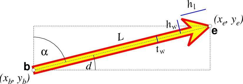
A GMT 4 vector has no separate pen for the stem -- it is all part of a Cartesian polygon. You may optionally fill and draw its outline. The modifiers listed above generally do not apply. Note: While the tailwidth (\(t_w\)) and headlength (\(h_l\)) parameters are given as indicated, the halfheadwidth (\(h_w\)) is oddly given as the half-width in GMT 4 so we retain that convention here (but have updated the documentation; blue lines indicate these three parameters).
Examples
Note: Below are some examples of valid syntax for this module.
The examples that use remote files (file names starting with @)
can be cut and pasted into your terminal for testing.
Other commands requiring input files are just dummy examples of the types
of uses that are common but cannot be run verbatim as written.
Note: Since many GMT plot examples are very short (i.e., one module call between the gmt begin and gmt end commands), we will often present them using the quick modern mode GMT Modern Mode One-line Commands syntax, which simplifies such short scripts.
To plot solid red circles (diameter = 0.2 cm) at the positions listed in the remote file DSDP.txt on a Mercator map at 0.3 cm/degree of the area 100E to 160E, 20S to 30N, with automatic tick-marks and gridlines:
gmt plot @DSDP.txt -R100/160/-20/30 -Jm0.3c -Sc0.2c -Gred -Bafg -pdf map
To plot the xyz values in the file quakes.xyzm as circles with size given by the magnitude in the 4th column and color based on the depth in the third using the CPT rgb.cpt on a linear map:
gmt plot quakes.xyzm -R0/1000/0/1000 -JX6i -Sc -Crgb -B200 -pdf map
To plot the file trench.txt on a Mercator map, with white triangles with sides 0.25 inch on the left side of the line, spaced every 0.8 inch:
gmt plot trench.txt -R150/200/20/50 -Jm0.15i -Sf0.8i/0.1i+l+t -Gwhite -W -B10 -pdf map
To plot a circle with color dictated by the t.cpt file for the z-value 65:
echo 175 30 | gmt plot -R150/200/20/50 -JM15c -B -Sc0.5c -Z65 -Ct.cpt -G+z -pdf map
To plot the data in the file misc.txt as symbols determined by the code in the last column, and with size given by the magnitude in the 4th column, and color based on the third column via the CPT chrome on a linear mape:
gmt plot misc.txt -R0/100/-50/100 -JX6i -S -Cchrome -B20 -pdf map
If you need to place vectors on a plot you can choose among straight Cartesian vectors, math circular vectors, or geo-vectors (these form small or great circles on the Earth). These can have optional heads at either end, and heads may be the traditional arrow, a circle, or a terminal cross-line. To place a few vectors with a circle at the start location and an arrow head at the end:
gmt plot -R0/50/-50/50 -JX6i -Sv0.15i+bc+ea -Gyellow -W0.5p -Baf -pdf map << EOF
10 10 45 2i
30 -20 0 1.5i
EOF
To plot vectors (red vector heads, solid stem) from the file data.txt that contains record of the form lon, lat, dx, dy, where dx, dy are the Cartesian vector components given in user units, and these user units should be converted to cm given the scale 3.60:
gmt plot -R20/40/-20/0 -JM6i -Sv0.15i+e+z3.6c -Gred -W0.25p -Baf data.txt -pdf map
Segment Header Parsing
Segment header records may contain one of more of the following options:
- -Gfill
Use the new fill and turn filling on
- -G-
Turn filling off
- -G
Revert to default fill (none if not set on command line)
- -Llabel
Set a label for this segment (e.g., perhaps for quoted lines)
- -Wpen
Use the new pen and turn outline on
- -W
Revert to default pen MAP_DEFAULT_PEN (if not set on command line)
- -W-
Turn outline off
- -Zzval
Obtain fill via cpt lookup using z-value zval (what the color is used for is controlled further by -L or -W)
- -ZNaN
Get the NaN color from the CPT
- -ttransparency
Obtain transparency and apply it to fill and pen colors.
Custom Symbols
GMT allows users to define and plot their own custom symbols. This is done by encoding the symbol using our custom symbol macro code described in Appendix N. Put all the macro codes for your new symbol in a file whose extension must be .def; you may then address the symbol without giving the extension (e.g., the symbol file tsunami.def is used by specifying -Sktsunami/size. The definition file can contain any number of plot code records, as well as blank lines and comment lines (starting with #). The module will look for the definition files in (1) the current directory, (2) the ~/.gmt directory, and (3) the $GMT_SHAREDIR/custom directory, in that order. Freeform polygons (made up of straight line segments and arcs of circles) can be designed - these polygons can be painted and filled with a pattern. Other standard geometric symbols can also be used. See Appendix Custom Plot Symbols for macro definitions.
GMT4 Vector
Note: The old-style, single-polygon vector available in GMT4 and earlier versions has been added to GMT5 for backwards compatibility with old scripts. For reference, the old vector syntax is listed here: The size, if present, will be interpreted as arrowwidth/headlength/headwidth. By default, arrow attributes remain invariant to the length of the arrow. To have the size of the vector scale down with decreasing length, append nnorm, so that vectors shorter than norm will have their dimensions scaled by the vector length divided by norm. To center the vector on the balance (mid) point, use -Svb; to align point with the vector head, use -Svh; to align point with the vector tail, use -Svt [Default]. If the input has the head point’s coordinates instead of direction and length, use -Svs. Upper case B, H, T, or S will draw a double-headed vector [Default is single head].
Polar Caps
We will automatically determine if a closed polygon is containing a geographic pole, i.e., being a polar cap. Such polygons requires special treatment under the hood to ensure proper filling. Many tools such as GIS packages are unable to handle polygons covering a pole and some cannot handle polygons crossing the Dateline. They work around this problem by splitting polygons into a west and east polygon or inserting artificial helper lines that makes a cut into the pole and back. Such doctored polygons may be misrepresented in GMT.
Bezier spline
The +s modifier to pen settings (-W) is limited to plotting lines and polygons. Lines with embellishments (fronts, decorated, or quoted lines) are excluded.
Auto-Legend
The -l option for symbols expects the symbol color, size, and type to be given on the command line. If you have variable symbol sizes then you must append +ssize to set a suitable size for the legend entry. For other symbol cases the -l option will be ignored. Legend entries also work for lines and polygons, but not more complicated features such as decorated and quoted lines, fronts, etc.
Data Column Order
The -S option determines how many size columns are required to generate the selected symbol, but if size is not given then we expect to read size from file. In addition, your use of options -H, -I and -t will require extra columns. The order of the data record is fixed regardless of option order, even if not all items may be activated. We expect data columns to come in the following order:
x y [z] [size-columns] [scale] [intens] [transp [transp2]] [trailing-text]
where items given in brackets are optional and under the control of the stated options: -C selects the optional z column for color-lookup, -S without a size selects the optional size-columns (may be more than one depending on the selected symbol), -H selects the optional scale column, -I selects the optional intens column, and -t selects the optional transp column(s). Trailing text is always optional. Notes: (1) If symbol code is not given by -S then it is expected to start the trailing text. (2) You can use -i to rearrange your data record to match the expected format.
Auto-legend entries
This module allows you to use the -l option to specify an automatic legend entry. This option is available for lines or symbols only. If the symbol size is variable and computed from other information (which may be true for some symbols deriving their size from other input columns), then you need to supply a representative legend size via the +S modifier.