14. Color Systems and Artificial Illumination
In this Chapter, we are going to try to explain the relationship between the RGB, CMYK, and HSV color systems so as to (hopefully) make them more intuitive. GMT allows users to specify colors in CPTs in either of these three systems. Interpolation between colors is performed in either RGB or HSV, depending on the specification in the CPT. Below, we will explain why this all matters.
14.1. RGB color system
Remember your (parents’) first color television set? Likely it had three little bright colored squares on it: red, green, and blue. And that is exactly what each color on the tube is made of: varying levels of red, green and blue light. Switch all of them off, r=g=b=0, then you have black. All of them at maximum, r=g=b=255, creates white. Your computer screen works the same way.
A mix of levels of red, green, and blue creates basically any color imaginable. In GMT each color can be represented by the triplet r7g7b. For example, 127/255/0 (half red, full green, and no blue) creates a color called chartreuse. The color sliders in the graphics program GIMP are an excellent way to experiment with colors, since they show you in advance how moving one of the color sliders will change the color. As Figure (a) of Chartreuse in GIMP shows: increase the red and you will get a more yellow color, while lowering the blue level will turn it into brown.
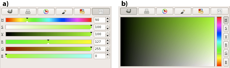
Chartreuse in GIMP. (a) Sliders indicate how the color is altered when changing the H, S, V, R, G, or B levels. (b) For a constant hue (here 90) value increases to the right and saturation increases up, so the pure color is on the top right.
Is chocolate your favorite color, but you do not know the RGB equivalent values? Then look them up in gmtcolors for a full list. It’s 210/105/30. But GMT makes it easy on you: you can specify pen, fill, and palette colors by any of the unique colors found in that file.
Are you very web-savvy and work best with hexadecimal color codes as
they are used in HTML? Even that is allowed in GMT. Just start with a
hash mark (#) and follow with the 2 hexadecimal characters for red,
green, and blue. For example, you can use #79ff00 for chartreuse,
#D2691E for chocolate.
14.2. HSV color system
If you have played around with RGB color sliders, you will have noticed that it is not intuitive to make a chosen color lighter or darker, more saturated or more gray. It would involve changing three sliders. To make it easier to manipulate colors in terms of lightness and saturation, another coordinate system was invented: HSV (hue, saturation, value). Those terms can be made clear best by looking at the color sliders in Figure Chartreuse in GIMPa. Hue (running from 0 to 360) gives you the full spectrum of saturated colors. Saturation (from 0 to 1, or 100%) tells you how ‘full’ your color is: reduce it to zero and you only have gray scales. Value (from 0 to 1, or 100%) will bring you from black to a fully saturated color. Note that “value” is not the same as “intensity”, or “lightness”, used in other color geometries. “Brilliance” may be the best alternative word to describe “value”. Apple calls it as “brightness”, and hence refers to HSB for this color space.
Want more chartreuse or chocolate? You can specify them in GMT as 90-1-1 and 25-0.86-0.82, respectively.
14.3. The color cube
We are going to try to give you a geometric picture of color mixing in RGB and HSV by means of a tour of the RGB cube depicted in Figure The RGB color cube. The geometric picture is most helpful, we think, since HSV are not orthogonal coordinates and not found from RGB by a simple algebraic transformation. So here goes: Look at the cube face with black, red, magenta, and blue corners. This is the g = 0 face. Orient the cube so that you are looking at this face with black in the lower left corner. Now imagine a right-handed cartesian (rgb) coordinate system with origin at the black point; you are looking at the g = 0 plane with r increasing to your right, g increasing away from you, and b increasing up. Keep this sense of (rgb) as you look at the cube.
Now tip the cube such that the black corner faces down and the white corner up. When looking from the top, you can see the hue, contoured in gray solid lines, running around in 360° counter-clockwise. It starts with shades of red (0), then goes through green (120) and blue (240), back to red.
On the three faces that are now on the lower side (with the white print) one of (rgb) is equal to 0. These three faces meet at the black corner, where r = g = b = 0. On these three faces the colors are fully saturated: s = 1. The dashed white lines indicate different levels of v, ranging from 0 to 1 with contours every 0.1.
On the upper three faces (with the black print), one of (rgb) is equal to the maximum value. These three faces meet at the white corner, where r = g = b = 255. On these three faces value is at its maximum: v = 1 (or 100%). The dashed black lines indicate varying levels of saturation: s ranges from 0 to 1 with contours every 0.1.
Now turn the cube around on its vertical axis (running from the black to the white corner). Along the six edges that zigzag around the “equator”, both saturation and value are maximum, so s = v = 1. Twirling the cube around and tracing the zigzag, you will visit six of the eight corners of the cube, with changing hue (h): red (0), yellow (60), green (120), cyan (180), blue (240), and magenta (300). Three of these are the RGB colors; the other three are the CMY colors which are the complement of RGB and are used in many color hardcopy devices (see below). The only cube corners you did not visit on this path are the black and white corners. They lie on the vertical axis where hue is undefined and r = g = b. Any point on this axis is a shade of gray.
Let us call the points where s = v = 1 (points along the RYGCBM path described above) the “pure” colors. If we start at a pure color and we want to whiten it, we can keep h constant and v = 1 while decreasing s; this will move us along one of the cube faces toward the white point. If we start at a pure color and we want to blacken it, we can keep h constant and s = 1 while decreasing v; this will move us along one of the cube faces toward the black point. Any point in (rgb) space which can be thought of as a mixture of pure color + white, or pure color + black, is on a face of the cube.
The points in the interior of the cube are a little harder to describe. The definition for h above works at all points in (non-gray) (rgb) space, but so far we have only looked at (s, v) on the cube faces, not inside it. At interior points, none of (rgb) is equal to either 0 or 255. Choose such a point, not on the gray axis. Now draw a line through your point so that the line intersects the gray axis and also intersects the RYGCBM path of edges somewhere. It is always possible to construct this line, and all points on this line have the same hue. This construction shows that any point in RGB space can be thought of as a mixture of a pure color plus a shade of gray. If we move along this line away from the gray axis toward the pure color, we are “purifying” the color by “removing gray”; this move increases the color’s saturation. When we get to the point where we cannot remove any more gray, at least one of (rgb) will have become zero and the color is now fully saturated; s = 1. Conversely, any point on the gray axis is completely undersaturated, so that s = 0 there. Now we see that the black point is special, s is both 0 and 1 at the same time. In other words, at the black point saturation in undefined (and so is hue). The convention is to use h = s = v = 0 at this point.
It remains to define value. To do so, try this: Take your point in RGB space and construct a line through it so that this line goes through the black point; produce this line from black past your point until it hits a face on which v = 1. All points on this line have the same hue. Note that this line and the line we made in the previous paragraph are both contained in the plane whose hue is constant. These two lines meet at some arbitrary angle which varies depending on which point you chose. Thus HSV is not an orthogonal coordinate system. If the line you made in the previous paragraph happened to touch the gray axis at the black point, then these two lines are the same line, which is why the black point is special. Now, the line we made in this paragraph illustrates the following: If your chosen point is not already at the end of the line, where v = 1, then it is possible to move along the line in that direction so as to increase (rgb) while keeping the same hue. The effect this has on a color monitor is to make the color more “brilliant”, your hue will become “stronger”; if you are already on a plane where at least one of (rgb) = 255, then you cannot get a stronger version of the same hue. Thus, v measures brilliance or strength. Note that it is not quite true to say that v measures distance away from the black point, because v is not equal to \(\sqrt{r^2 + g^2 + b^2}/255\).
Another representation of the HSV space is the color cone illustrated in Figure The HSV color space.
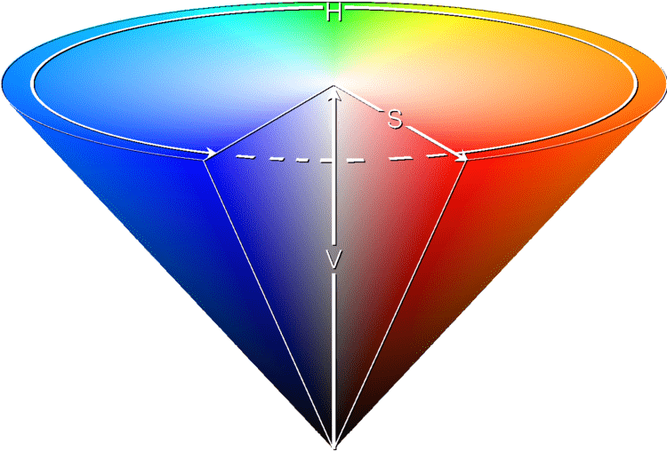
The HSV color space
14.4. Color interpolation
From studying the RGB cube, we hope you will have understood that there are different routes to follow between two colors, depending whether you are in the RGB or HSV system. Suppose you would make an interpolation between blue and red. In the RGB system you would follow a path diagonally across a face of the cube, from 0/0/255 (blue) via 127/0/127 (purple) to 255/0/0 (red). In the HSV system, you would trace two edges, from 240-1-1 (blue) via 300-1-1 (magenta) to 360-1-1 (red). That is even assuming software would be smart enough to go the shorter route. More likely, red will be recorded as 0-1-1, so hue will be interpolated the other way around, reducing hue from 240 to 0, via cyan, green, and yellow.
Depending on the design of your CPT, you may want to have it
either way. By default, GMT interpolates in RGB space, even when the
original CPT is in the HSV system. However, when you add the
line #COLOR_MODEL=+HSV (with the leading ‘+’ sign) in the header of
the CPT, GMT will not only read the color
representation as HSV values, but also interpolate colors in the HSV
system. That means that H, S, and V values are interpolated linearly
between two colors, instead of their respective R, G, and B values.
The top row in Figure Interpolating colors illustrates two examples: a blue-white-red scale (the palette in Chapter Of Colors and Color Legends) interpolated in RGB and the palette interpolated in HSV. The bottom row of the Figure demonstrates how things can go terribly wrong when you do the interpolation in the other system.
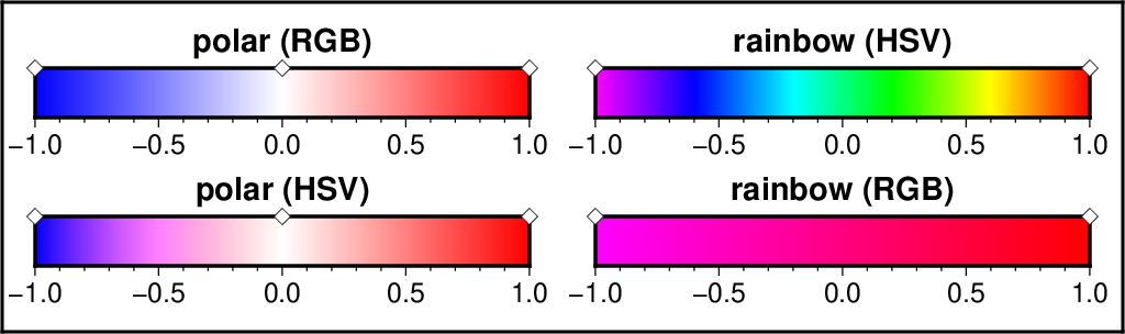
When interpolating colors, the color system matters. The polar palette on the left needs to be interpolated in RGB, otherwise hue will change between blue (240) and white (0). The rainbow palette should be interpolated in HSV, since only hue should change between magenta (300) and red (0). Diamonds indicate which colors are defined in the palettes; they are fixed, the rest is interpolated.
Here is the source script for the figure above:
gmt begin GMT_color_interpolate
	gmt set GMT_THEME cookbook
	gmt basemap -Jx1i -R0/6.8/0/2.0 -B0

	gmt makecpt -Cpolar -T-1/1
	gmt colorbar -Dx1.7/1.6+w3i/0.3i+h+jTC -C -B0.5f0.1
	gmt colorbar -Dx1.7/0.7+w3i/0.3i+h+jTC -C -B0.5f0.1 --COLOR_MODEL=hsv

	gmt makecpt -Crainbow -T-1/1
	gmt colorbar -Dx5.1/1.6+w3i/0.3i+h+jTC -C -B0.5f0.1
	gmt colorbar -Dx5.1/0.7+w3i/0.3i+h+jTC -C -B0.5f0.1 --COLOR_MODEL=rgb

	gmt plot -Sd0.1i -Wblack -Gwhite << END
0.2 1.6
1.7 1.6
3.2 1.6
3.6 1.6
6.6 1.6
0.2 0.7
1.7 0.7
3.2 0.7
3.6 0.7
6.6 0.7
END

	gmt text -F+f14p,Helvetica-Bold+jBC << END
1.7 1.7 polar (RGB)
1.7 0.8 polar (HSV)
5.1 1.7 rainbow (HSV)
5.1 0.8 rainbow (RGB)
END
gmt end show
14.5. Artificial illumination
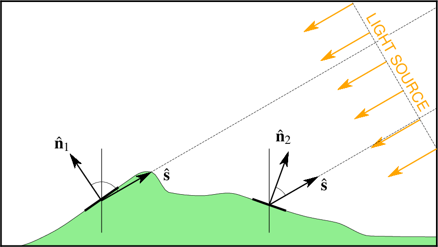
For digital elevation models (DEM) one can specify an illumination azimuth and elevation and compute the unit vector s. Then, at any point on the grid we can compute the normal vector n. Their dot products can be used to compute an intensity grid that will be positive if the surface faces the light, negative if facing away, and zero if the vectors are orthogonal. In GMT, uses may wish to add artificial illumination on non-DEM data, such as geopotential data. In those cases, while an illumination azimuth still makes sense, an elevation does not since the normal vectors no longer can easily be related to elevation. GMT thus only uses the directions of these vectors and normalizes the intensities to yield suitable shading; see grdgradient for more details.
Here is the source script for the figure above:
cat << EOF > t.txt
0	0
1	1
1.2	1.03
2	1
3	1.25
4	1.8
5	2.5
6	3.2
6.5	3.3
7	2.7
8	2.6
9	2.65
10	2.3
11	2
12	1.8
13	1.4
14	1.38
15	1.37
EOF
gmt sample1d -I0.1 t.txt -Fa > t2.txt
cat << EOF >> t2.txt
15	1.371
15	0
0	0
EOF
gmt begin GMT_slope2intensity
	gmt set GMT_THEME cookbook
	gmt plot -R2/15/1.1/8.4 -Jx0.44444i -B0 t2.txt -Glightgreen -W0.25p
	gmt plot -Sv14p+e+jb+h0.5 -W1p,orange -Gorange -N <<- EOF
	15	4	210	0.75i
	14.5	4.866	210	0.75i
	14	5.732	210	0.75i
	13.5	6.598	210	0.75i
	13	7.4641	210	0.75i
	12.5	8.330	210	0.75i
	EOF
	gmt plot -W2p <<- EOF
	> left
	4.5	2.15
	5.5	2.85
	> right
	9.5	2.5
	10.5	2.15
	> v1 -W0.5p
	5	4
	5	1.5
	> v2 -W0.5p
	10	4
	10	1.5
	> sun -W0.25p,-
	15	4
	10	12.66025
	> line to sun -W0.25p,-
	5	2.45
	15	8.2235
	> line to sun -W0.25p,-
	10	2.325
	15	5.2118
	EOF
	gmt plot -Sv14p+e+h0.5 -W1p -Gblack -N <<- EOF
	5	2.45	124	0.75i
	5	2.45	30	0.75i
	10	2.325	70	0.75i
	10	2.325	30	0.75i
	EOF
	gmt plot -Sw0.5i -W0.25p -N <<- EOF
	5	2.45	30	124
	10	2.325	30	70
	EOF
	echo 	13.7	6.5	-60	14p,Helvetica,orange	CB	LIGHT SOURCE | gmt text -F+a+f+j -Gwhite -C0
	gmt text -F+a+f+j <<- EOF
	4.1		3.9	0	16p,Times-Roman	RB	<math>\\hat{\\mathbf{n}}_1</math>
	10.7	4.1	0	16p,Times-Roman	RB	<math>\\hat{\\mathbf{n}}_2</math>
	11.5	2.7	0	16p,Times-Roman	LB	<math>\\hat{\\mathbf{s}}</math>
	6.8		3.0	0	16p,Times-Roman	LB	<math>\\hat{\\mathbf{s}}</math>
	EOF
gmt end show
rm -f t.txt t2.txt
GMT uses the HSV system to achieve artificial illumination of colored images (e.g., -I option in grdimage) by changing the saturation s and value v coordinates of the color. As explained above, when the intensity is zero (flat illumination), the data are colored according to the CPT. If the intensity is non-zero, the color is either lightened or darkened depending on the illumination. The color is first converted to HSV (if necessary) and then darkened by moving (sv) toward (COLOR_HSV_MIN_S, COLOR_HSV_MIN_V) if the intensity is negative, or lightened by sliding (sv) toward (COLOR_HSV_MAX_S, COLOR_HSV_MAX_V) if the illumination is positive. The extremes of the s and v are defined in the gmt.conf file and are usually chosen so the corresponding points are nearly black (s = 1, v = 0) and white (s = 0, v = 1). The reason this works is that the HSV system allows movements in color space which correspond more closely to what we mean by “tint” and “shade”; an instruction like “add white” is easy in HSV and not so obvious in RGB.
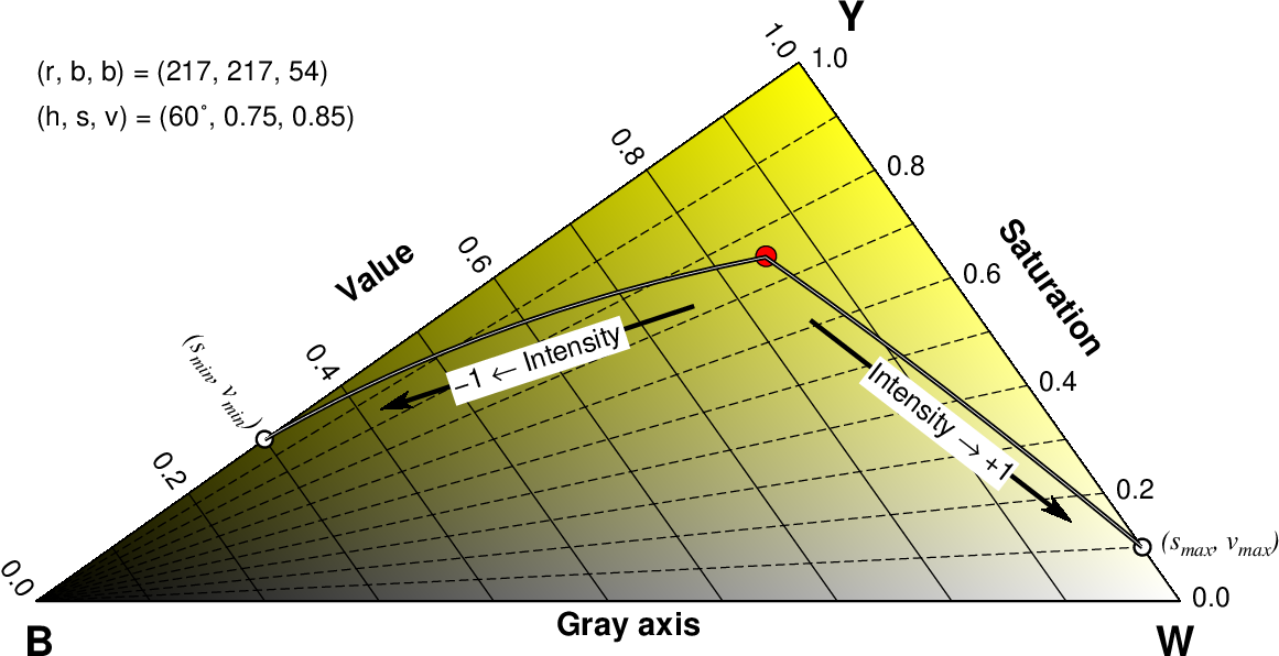
The red circle represents the RGB color (217, 271, 54). This color has a hue that is yellow, which is H = 60 degrees in the HSV system. Here we show a slice through the color RGB cube at H = 60. All the colors in this slice have a yellow hue but there saturation and values vary. Our point has an S of 0.75 and a V of 0.85. In applications that take intensity values we use an intensity (in the range of ±1) to move the color towards the black (B) or white (W) point for negative and positive intensities, respectively (an intensity of 0 leaves the color unchanged). Because (a) printers are not good at yielding near-black or near-white colors, and (2) to avoid colors with saturating intensities being pushed into black and white, we do not use the B and W points as terminal points but instead end at the two white circles. Their coordinates are given by (COLOR_HSV_MIN_S, COLOR_HSV_MIN_V) [1, 0.3] and (COLOR_HSV_MAX_S, COLOR_HSV_MAX_V) [0.1, 1].
Here is the source script for the figure above:
ps=GMT_color_hsv.ps
x=4
r=217
b=54
smin=1.0
smax=0.1
vmin=0.3
vmax=1.0
y=`gmt math -Q $x 2 SQRT MUL =`
gmt grdmath -I1 -R0/255/0/255 Y 256 MUL X ADD = rgb_cube.grd
gmt grdmath -I1 -R0/255/0/255 Y 255 DIV = v.grd
gmt grdmath -I1 -R0/255/0/255 1 X Y DIV SUB X Y LE MUL = s.grd
gmt math -T0/255/1 -N3/0  T 256 MUL 0.5 SUB -C2 256 ADD  = | awk '{printf "%s\t%d/%d/0\t%s\t%d/%d/255\n", $2, $1, $1, $3, $1, $1}' > rgb_cube.cpt
gmt psxy -R0/8/0/8 -Jx1i -P -K -X0.75i -Y2i -T > $ps
cat << EOF >> $ps
gsave
-54.735611 rotate
EOF
cat << EOF > path.txt
0	0
255	255
0	255
0	0
EOF
gmt psclip -R0/255/0/255 -JX${x}i/${y}i path.txt -O -K >> $ps
gmt grdimage rgb_cube.grd -Crgb_cube.cpt -JX -O -K >> $ps
cat << EOF > t.txt
0.1	C
0.3	C
0.5	C
0.7	C
0.9	C
EOF
gmt grdcontour v.grd -C0.1 -Gd1 -W0.5p -JX -O -K >> $ps
gmt grdcontour s.grd -C0.1 -Gd1 -W0.5p,- -JX -O -K >> $ps
gmt psclip -O -K -C >> $ps
gmt pstext -R -JX -O -K -N -Dj0.06i << EOF >> $ps
0	-7	18	54.735611	1	LT	B
252	245	18	54.735611	1	LT	W
5	270	18	54.735611	1	CB	Y
0	260	12	0	0	RT	1.0
0	209	12	0	0	RT	0.8
0	158	12	0	0	RT	0.6
0	107	12	0	0	RT	0.4
-2	82	12	0	6	RT	(s@-min@-, v@-min@-)
0	56	12	0	0	RT	0.2
0	5	12	0	0	RT	0.0
235	255	12	54.735611	6	LB	(s@-max@-, v@-max@-)
260	253	12	54.735611	0	LB	0.0
209	253	12	54.735611	0	LB	0.2
158	253	12	54.735611	0	LB	0.4
107	253	12	54.735611	0	LB	0.6
56	253	12	54.735611	0	LB	0.8
5	253	12	54.735611	0	LB	1.0
-20	127.5	14	90		1	CB	Value
127.5	270	14	0		1	BC	Saturation
146	125	14	54.7356		1	BC	Gray axis
-80	150	12	54.735611	0	RM	(h, s, v) = (60\232, 0.75, 0.85)
-100	151	12	54.735611	0	RM	(r, b, b) = (217, 217, 54)
EOF
gmt psxy -R -JX -O -K -W1p path.txt >> $ps
echo "$b $r" | gmt psxy -R -JX -O -K -Sc9p -Gred -W0.5p >> $ps
gmt math -T-1/0/0.01 0.75 $smin SUB T MUL 0.75 ADD = saturation.txt
gmt math -T0/1/0.01 $smax 0.75 SUB T MUL 0.75 ADD = >> saturation.txt
gmt math -T-1/0/0.01 0.85 $vmin SUB T MUL 0.85 ADD = value.txt
gmt math -T0/1/0.01 $vmax 0.85 SUB T MUL 0.85 ADD = >> value.txt
cat << EOF | gmt math STDIN HSV2RGB = | awk '{print $3, $1}' | gmt psxy -R -JX -O -K -W1p -Sc0.1i -Gwhite -N >> $ps
60	$smax	$vmax
60	$smin	$vmin
EOF
paste saturation.txt value.txt | awk '{print 60, $2, $4}' | gmt math STDIN HSV2RGB = | awk '{print $3, $1}' > curve.txt
gmt  psxy -R -JX -O -K -W2p curve.txt >> $ps
gmt  psxy -R -JX -O -K -W0.25p,white curve.txt >> $ps
gmt  psxy -R -JX -O -K -Sv14p+e+jc+h0.5 -G0 -W2p << EOF >> $ps
145 230 17 2i
35	150 -107 2i
EOF
gmt pstext -R -JX -O -K -N -Dj0.05/0.05 -Gwhite << EOF >> $ps
145	230	12	17	0	MC	Intensity @~\256@~ +1
35	150	12	73	0	MC	\0551 @~\254@~ Intensity
EOF
echo "grestore" >> $ps
gmt psxy -R -JX -O -T >> $ps
rm -f t.txt s.grd v.grd rgb_cube.cpt rgb_cube.grd curve.txt path.txt saturation.txt value.txt
14.6. Thinking in RGB or HSV
The RGB system is understandable because it is cartesian, and we all learned cartesian coordinates in school. But it doesn’t help us create a tint or shade of a color; we cannot say, “We want orange, and a lighter shade of orange, or a less vivid orange”. With HSV we can do this, by saying, “Orange must be between red and yellow, so its hue is about h = 30; a less vivid orange has a lesser s, a darker orange has a lesser v”. On the other hand, the HSV system is a peculiar geometric construction, more like a cone (Figure The HSV color space). It is not an orthogonal coordinate system, and it is not found by a matrix transformation of RGB; these make it difficult in some cases too. Note that a move toward black or a move toward white will change both s and v, in the general case of an interior point in the cube. The HSV system also doesn’t behave well for very dark colors, where the gray point is near black and the two lines we constructed above are almost parallel. If you are trying to create nice colors for drawing chocolates, for example, you may be better off guessing in RGB coordinates.
14.7. CMYK color system
Finally, you can imagine that printers work in a different way: they mix different paints to make a color. The more paint, the darker the color, which is the reverse of adding more light. Also, mixing more colored paints does not give you true black, so that means that you really need four colors to do it right. Open up your color printer and you’ll probably find four cartridges: cyan, magenta, yellow (often these are combined into one), and black. They form the CMYK system of colors, each value running from 0 to 1 (or 100%). In GMT CMYK color coding can be achieved using c/m/y/k quadruplets.
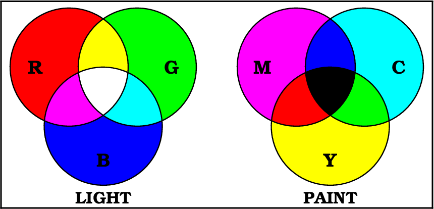
(left) Mixing of light on a computer screen shows that the mixing of primary colors red (R), green (G) and blue (B) yields the other primary colors of magenta (M), cyan (C) and yellow (Y), plus white. (right) Mixing of colors for printing uses C, M and Y and when these mix completely we get black (K). To get a better representation of black the amount of black in any particular color is removed from the color and painted with a specific black ink instead, leading to under-color removal of the remaining three pigments.
Here is the source script for the figure above:
gmt project -N -Z2.6+e -G0.02 -C-0.75/1.3 > R.d
gmt project -N -Z2.6+e -G0.02 -C0.75/1.3  > G.d
gmt project -N -Z2.6+e -G0.02 -C0/0       > B.d
gmt project -N -Z2.6+e -G0.02 -C4.25/1.3  > M.d
gmt project -N -Z2.6+e -G0.02 -C5.75/1.3  > C.d
gmt project -N -Z2.6+e -G0.02 -C5/0       > Y.d

gmt begin GMT_cmyk
	gmt set GMT_THEME cookbook
	gmt plot -R-2.25/7.25/-1.8/2.75 -Jx0.6i R.d -Gred -B0
	gmt plot G.d -Ggreen
	gmt plot B.d -Gblue
	gmt plot C.d -Gcyan
	gmt plot M.d -Gmagenta
	gmt plot Y.d -Gyellow
	# Do R&G
	gmt convert R.d G.d | gmt clip -N
	gmt plot G.d -Gyellow
	gmt clip -C
	# Do R&B
	gmt convert R.d B.d | gmt clip -N
	gmt plot R.d -Gmagenta
	gmt clip -C
	# Do G&B
	gmt convert G.d B.d | gmt clip -N
	gmt plot G.d -Gcyan
	gmt clip -C
	# Do W
	gmt select -FR.d B.d | gmt select -FG.d > b.txt
	gmt select -FR.d G.d | gmt select -FB.d > g.txt
	gmt select -FB.d R.d | gmt select -FG.d > r.txt
	cat r.txt b.txt g.txt | gmt plot -Gwhite
	# Do C&M
	gmt convert C.d M.d | gmt clip -N
	gmt plot C.d -Gblue
	gmt clip -C
	# Do C&Y
	gmt convert C.d Y.d | gmt clip -N
	gmt plot C.d -Ggreen
	gmt clip -C
	# Do M&Y
	gmt convert M.d Y.d | gmt clip -N
	gmt plot M.d -Gred
	gmt clip -C
	# Do K
	gmt select -FC.d Y.d | gmt select -FM.d > y.txt
	gmt select -FC.d M.d | gmt select -FY.d > m.txt
	gmt select -FY.d C.d | gmt select -FM.d > c.txt
	cat c.txt y.txt m.txt | gmt plot -Gblack
	gmt plot [GRBCMY].d -W1p
	gmt text -F+f16p,Bookman-Demi+jBC <<- EOF
	0		-1.7	LIGHT
	5		-1.7	PAINT
	EOF
	gmt text -F+f18p,Bookman-Demi+jCM <<- EOF
	-1.5	1.3		R
	1.5		1.3		G
	0		-0.75	B
	3.5		1.3		M
	6.5		1.3		C
	5		-0.75	Y
	EOF
gmt end show
rm -f [GRBCMY].d [rgbcmy].txt
Obviously, there is no unique way to go from the 3-dimensional RGB system to the 4-dimensional CMYK system. So, again, there is a lot of hand waving applied in the transformation. Strikingly, CMYK actually covers a smaller color space than RGB. We will not try to explain you the details behind it, just know that there is a transformation needed to go from the colors on your screen to the colors on your printer. It might explain why what you see is not necessarily what you get. If you are really concerned about how your color plots will show up in your PhD thesis, for example, it might be worth trying to save and print all your color plots using the CMYK system. Letting GMT do the conversion to CMYK may avoid some nasty surprises when it comes down to printing. To specify the color space of your PostScript file, set PS_COLOR_MODEL in the gmt.conf file to RGB, HSV, or CMYK.