6. GMT Map Projections

GMT implements more than 30 different projections. They all project the input coordinates longitude and latitude to positions on a map. In general, \(x' = f(x,y,z)\) and \(y' = g(x,y,z)\), where \(z\) is implicitly given as the radial vector length to the \((x,y)\) point on the chosen ellipsoid. The functions \(f\) and \(g\) can be quite nasty and we will refrain from presenting details in this document. The interested reader is referred to Snyder [1987][20]. We will mostly be using the coast command to demonstrate each of the projections. GMT map projections are grouped into four categories depending on the nature of the projection. The groups are

1. Conic projections

2. Azimuthal projections

3. Cylindrical projections

4. Miscellaneous projections

Because \(x\) and \(y\) are coupled we can only specify one plot-dimensional scale, typically a map scale (for lower-case map projection code) or a map width (for upper-case map projection code). The measurement unit is cm, inch, or point, depending on the PROJ_LENGTH_UNIT setting in gmt.conf, but this can be overridden on the command line by appending c, i, or p to the scale or width values. In some cases it would be more practical to specify map height instead of width, while in other situations it would be nice to set either the shortest or longest map dimension. Users may select these alternatives by appending a character code to their map dimension [detault is +dw]:

• Append +dh to the given dimension to specify map height.

• Append +du to the given dimension to select the minimum map dimension.

• Append +dl to the given dimension to select the maximum map dimension.

The ellipsoid used in map projections is user-definable. 73 commonly used ellipsoids and spheroids are currently supported, and users may also specify their own custom ellipsoid parameters [default is WGS-84]. Several GMT parameters can affect the projection: PROJ_ELLIPSOID, GMT_INTERPOLANT, PROJ_SCALE_FACTOR, and PROJ_LENGTH_UNIT; see the gmt.conf man page for details.

In GMT version 4.3.0 we noticed we ran out of the alphabet for 1-letter (and sometimes 2-letter) projection codes. To allow more flexibility, and to make it easier to remember the codes, we implemented the option to use the abbreviations used by the PROJ mapping package. Since some of the GMT projections are not in PROJ, we invented some of our own as well. For a full list of both the old 1- and 2-letter codes, as well as the PROJ-equivalents see the quick reference table below. For example, -JM15c and -JMerc/15c have the same meaning.

Projection	GMT CODES	PROJ CODES	Parameters
	-J (scale|WIDTH);	-J (scale)
Lambert azimuthal equal area	-Ja|A	-Jlaea/	lon0/lat0[/horizon]/scale|width
Albers conic equal area	-Jb|B	-Jaea/	lon0/lat0/lat1/lat2/scale|width
Cassini cylindrical	-Jc|C	-Jcass/	lon0/lat0/scale|width
Cylindrical stereographic	-Jcyl_stere|Cyc_stere	-Jcyl_stere/	[lon0[/lat0]/]scale|width
Equidistant conic	-Jd|D	-Jeqdc/	lon0/lat0/lat1/lat2/scale|width
Azimuthal equidistant	-Je|E	-Jaeqd/	lon0/lat0[/horizon]/scale|width
Azimuthal gnomonic	-Jf|F	-Jgnom/	lon0/lat0[/horizon]/scale|width
Azimuthal orthographic	-Jg|G	-Jortho/	lon0/lat0[/horizon]/scale|width
General perspective	-Jg|G	-Jnsper/	lon0/lat0/scale|width[+aazimuth][+ttilt][+vvwidth/vheight][+wtwist][+zaltitude[r|R]|g]
Hammer equal area	-Jh|H	-Jhammer/	lon0/scale|width
Sinusoidal equal area	-Ji|I	-Jsinu/	lon0/scale|width
Miller cylindrical	-Jj|J	-Jmill/	lon0/scale|width
Eckert IV equal area	-Jkf|Kf	-Jeck4/	lon0/scale|width
Eckert VI equal area	-Jks|Ks	-Jeck6/	lon0/scale|width
Lambert conic conformal	-Jl|L	-Jlcc/	lon0/lat0/lat1/lat2/scale|width
Mercator cylindrical	-Jm|M	-Jmerc/	[lon0[/lat0/]]scale|width
Robinson	-Jn|N	-Jrobin/	[lon0/]scale|width
Oblique Mercator, 1: origin and azim	-Jo|O[a|A]	-Jomerc/	lon0/lat0/azim/scale|width [+v]
Oblique Mercator, 2: two points	-Jo|O[b|B]	-Jomerc/	lon0/lat0/lon1/lat1/scale|width[+v]
Oblique Mercator, 3: origin and pole	-Jo|O[c|C]	-Jomercp/	lon0/lat0/lonp/latp/scale|width[+v]
Polar [azimuthal] (\(\theta, r\)) (or cylindrical)	-Jp|P	-Jpolar/	scale|width[+a][+f[e|p|radius]][+kkind][+roffset][+torigin][+z[p|radius]]
(American) polyconic	-Jpoly|Poly	-Jpoly/	[lon0[/lat0/]]scale|width
Equidistant cylindrical	-Jq|Q	-Jeqc/	[lon0[/lat0/]]scale|width
Winkel Tripel	-Jr|R	-Jwintri/	[lon0/]scale|width
General stereographic	-Js|S	-Jstere/	lon0/lat0[/horizon]/scale|width
Transverse Mercator	-Jt|T	-Jtmerc/	[lon0[/lat0/]]scale|width
Universal Transverse Mercator (UTM)	-Ju|U	-Jutm/	zone/scale|width
Van der Grinten	-Jv|V	-Jvandg/	[lon0/]scale|width
Mollweide	-Jw|W	-Jmoll/	[lon0/]scale|width
Linear, logarithmic, power, and time	-Jx|X	-Jxy	xscale|width[l|ppower|T|t][/yscale|height[l|ppower|T|t]][d]
Cylindrical equal area	-Jy|Y	-Jcea/	lon0/lat0/scale|width

6.1. Conic projections

6.1.1. Albers conic equal-area projection (-Jb -JB)

Syntax

-Jb|Blon0/lat0/lat1/lat2/scale|width

Parameters

• The longitude (lon0) and latitude (lat0) of the projection center.

• The two standard parallels (lat1 and lat2).

• The scale in plot-units/degree or as 1:xxxxx (with -Jb) or map width in plot-units (with -JB).

Note that you must include the “1:” if you choose to specify the scale that way. For example, you can say 0.5c which means 0.5 cm/degree or 1:200000 which means 1 unit on the map equals 200,000 units along the standard parallels. The projection center defines the origin of the rectangular map coordinates.

Description

This projection, developed by Heinrich C. Albers in 1805, is predominantly used to map regions of large east-west extent, in particular the United States. It is a conic, equal-area projection, in which parallels are unequally spaced arcs of concentric circles, more closely spaced at the north and south edges of the map. Meridians, on the other hand, are equally spaced radii about a common center, and cut the parallels at right angles. Distortion in scale and shape vanishes along the two standard parallels. Between them, the scale along parallels is too small; beyond them it is too large. The opposite is true for the scale along meridians.

Example

As an example we will make a map of the region near Taiwan. We choose the center of the projection to be at 125°E/20°N and 25°N and 45°N as our two standard parallels. We desire a map that is 12 cm wide. The complete command needed to generate the map below is therefore given by:

gmt begin GMT_albers
	gmt set GMT_THEME cookbook
	gmt set MAP_GRID_CROSS_SIZE_PRIMARY 0
	gmt coast -R110/140/20/35 -JB125/20/25/45/12c -Bag -Dl -Ggreen -Wthinnest -A250
gmt end show

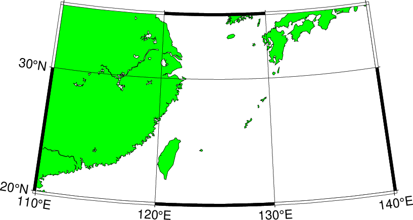
Albers equal-area conic map projection.

6.1.2. Equidistant conic projection (-Jd -JD)

Syntax

-Jd|Dlon0/lat0/lat1/lat2/scale|width

Parameters

• The longitude (lon0) and latitude (lat0) of the projection center.

• The two standard parallels (lat1 and lat2).

• The scale in plot-units/degree or as 1:xxxxx (with -Jd) or map width in plot-units (with -JD).

Description

The equidistant conic projection was described by the Greek philosopher Claudius Ptolemy about A.D. 150. It is neither conformal or equal-area, but serves as a compromise between them. The scale is true along all meridians and the standard parallels.

Example

The equidistant conic projection is often used for atlases with maps of small countries. As an example, we generate a map of Cuba:

gmt begin GMT_equidistant_conic
	gmt set GMT_THEME cookbook
	gmt set FORMAT_GEO_MAP ddd:mm:ssF MAP_GRID_CROSS_SIZE_PRIMARY 0.15c
	gmt coast -R-88/-70/18/24 -JD-79/21/19/23/12c -Bag -Di -N1/thick,red -Glightgreen -Wthinnest
gmt end show

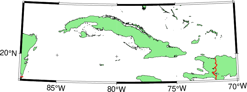
Equidistant conic map projection.

6.1.3. Lambert conic conformal projection (-Jl -JL)

Syntax

-Jl|Llon0/lat0/lat1/lat2/scale|width

Parameters

• The longitude (lon0) and latitude (lat0) of the projection center.

• The two standard parallels (lat1 and lat2).

• The scale in plot-units/degree or as 1:xxxxx (with -Jl) or map width in plot-units (with -JL).

Description

This conic projection was designed by the Alsatian mathematician Johann Heinrich Lambert (1772) and has been used extensively for mapping of regions with predominantly east-west orientation, just like the Albers projection. Unlike the Albers projection, Lambert’s conformal projection is not equal-area. The parallels are arcs of circles with a common origin, and meridians are the equally spaced radii of these circles. As with Albers projection, it is only the two standard parallels that are distortion-free.

Example

The Lambert conformal projection has been used for basemaps for all the 48 contiguous States with the two fixed standard parallels 33°N and 45°N. We will generate a map of the continental USA using these parameters. Note that with all the projections you have the option of selecting a rectangular border rather than one defined by meridians and parallels. Here, we choose the regular WESN region, a “fancy” basemap frame, and use degrees west for longitudes. The generating commands used were:

gmt begin GMT_lambert_conic
	gmt set GMT_THEME cookbook
	gmt set MAP_FRAME_TYPE FANCY FORMAT_GEO_MAP ddd:mm:ssF MAP_GRID_CROSS_SIZE_PRIMARY 0.15c
	gmt coast -R-130/-70/24/52 -Jl-100/35/33/45/1:50000000 -Bag -Dl -N1/thick,red -N2/thinner -A500 -Gtan -Wthinnest,white -Sblue
gmt end show

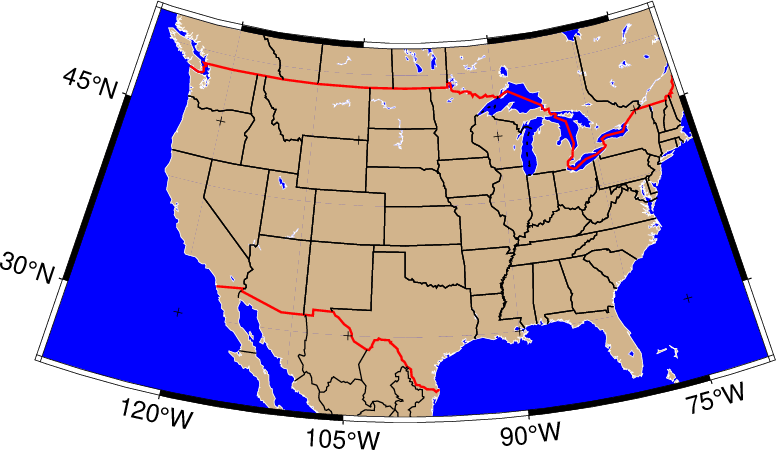
Lambert conformal conic map projection.

The choice for projection center does not affect the projection but it indicates which meridian (here 100°W) will be vertical on the map. The standard parallels were originally selected by Adams to provide a maximum scale error between latitudes 30.5°N and 47.5°N of 0.5–1%. Some areas, like Florida, experience scale errors of up to 2.5%.

6.1.4. (American) polyconic projection (-Jpoly -JPoly)

Syntax

-Jpoly|Poly/[lon0/[lat0/]]scale|width

Parameters

• The longitude (lon0) and latitude (lat0) of the projection center.

• The two standard parallels (lat1 and lat2).

• The scale in plot-units/degree or as 1:xxxxx (with -Jl) or map width in plot-units (with -JL).

Description

The polyconic projection, in Europe usually referred to as the American polyconic projection, was introduced shortly before 1820 by the Swiss-American cartographer Ferdinand Rodulph Hassler (1770–1843). As head of the Survey of the Coast, he was looking for a projection that would give the least distortion for mapping the coast of the United States. The projection acquired its name from the construction of each parallel, which is achieved by projecting the parallel onto the cone while it is rolled around the globe, along the central meridian, tangent to that parallel. As a consequence, the projection involves many cones rather than a single one used in regular conic projections.

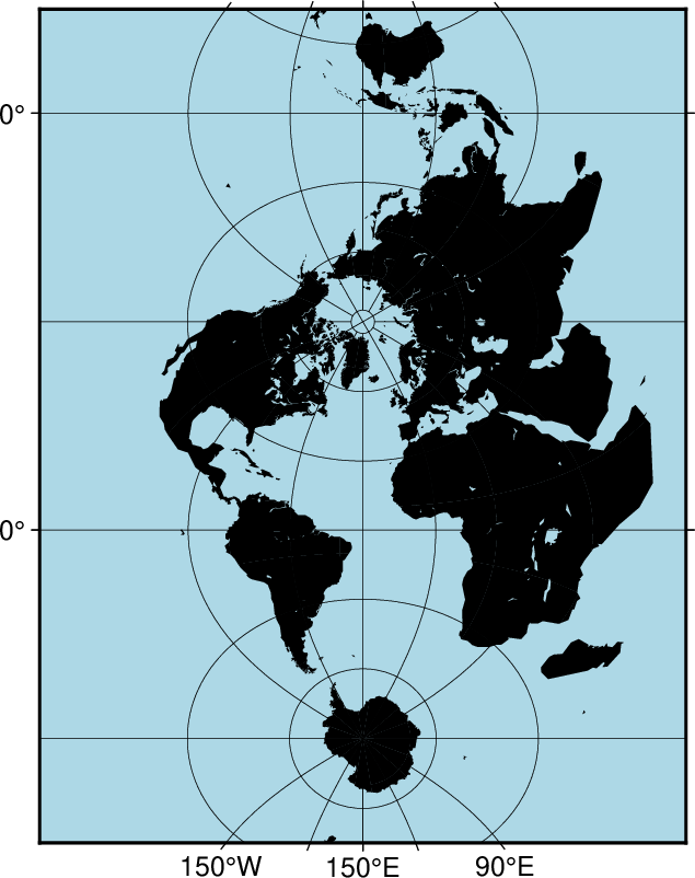
The polyconic projection is neither equal-area, nor conformal. It is true to scale without distortion along the central meridian. Each parallel is true to scale as well, but the meridians are not as they get further away from the central meridian. As a consequence, no parallel is standard because conformity is lost with the lengthening of the meridians.

Example

Below we reproduce the illustration by Snyder [1987], with a gridline every 10 and annotations only every 30° in longitude:

gmt coast -R-180/-20/0/90 -JPoly/10c -Bx30g10 -By10g10 -Dc -A1000 -Glightgray -Wthinnest --GMT_THEME=cookbook -view GMT_polyconic

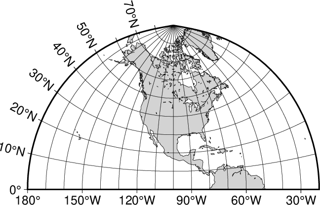
(American) polyconic projection.

6.2. Azimuthal projections

6.2.1. Lambert Azimuthal Equal-Area (-Ja -JA)

Syntax

-Ja|Alon0/lat0[/horizon]scale|width

Parameters

• The longitude (lon0) and latitude (lat0) of the projection center.

• Optionally, the horizon, i.e., the number of degrees from the center to the edge (<=180) [default is 90].

• The scale as 1:xxxxx or as radius/latitude where radius is the projected distance on the map from projection center to an oblique latitude where 0 would be the oblique Equator (with -Ja) or map width plot-units (with -JA).

Description

This projection was developed by Johann Heinrich Lambert in 1772 and is typically used for mapping large regions like continents and hemispheres. It is an azimuthal, equal-area projection, but is not perspective. Distortion is zero at the center of the projection, and increases radially away from this point.

Examples

Two different types of maps can be made with this projection depending on how the region is specified. We will give examples of both types in the next two subsections.

6.2.1.1. Rectangular map

In this mode we define our region by specifying the longitude/latitude of the lower left and upper right corners instead of the usual west, east, south, north boundaries. The reason for specifying our area this way is that for this and many other projections, lines of equal longitude and latitude are not straight lines and are thus poor choices for map boundaries. Instead we require that the map boundaries be rectangular by defining the corners of a rectangular map boundary. Using 0°E/40°S (lower left) and 60°E/10°S (upper right) as our corners we try

gmt begin GMT_lambert_az_rect
	gmt set GMT_THEME cookbook
	gmt set FORMAT_GEO_MAP ddd:mm:ssF MAP_GRID_CROSS_SIZE_PRIMARY 0
	gmt coast -R0/-40/60/-10+r -JA30/-30/12c -Bag -Dl -A500 -Gp10+r300 -Wthinnest
gmt end show

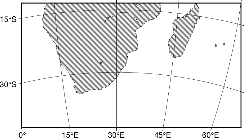
Rectangular map using the Lambert azimuthal equal-area projection.

Note that an +r is appended to the -R option to inform GMT that the region has been selected using the rectangle technique, otherwise it would try to decode the values as west, east, south, north and report an error since ‘east’ < ‘west’.

6.2.1.2. Hemisphere map

Here, you must specify the world as your region (-Rg or -Rd). E.g., to obtain a hemisphere view that shows the Americas, try

gmt coast -Rg -JA280/30/12c -Bg -Dc -A1000 -Gnavy --GMT_THEME=cookbook -view GMT_lambert_az_hemi

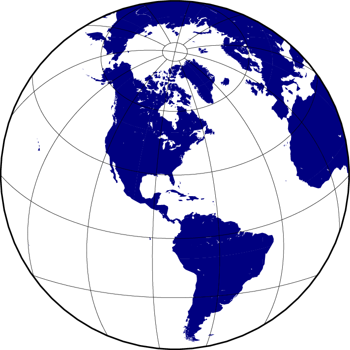
Hemisphere map using the Lambert azimuthal equal-area projection.

To geologists, the Lambert azimuthal equal-area projection (with origin at 0/0) is known as the equal-area (Schmidt) stereonet and used for plotting fold axes, fault planes, and the like. An equal-angle (Wulff) stereonet can be obtained by using the stereographic projection (discussed later). The stereonets produced by these two projections appear below.

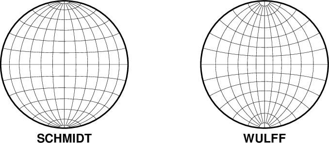
Equal-Area (Schmidt) and Equal-Angle (Wulff) stereo nets.

Here is the source script for the figure above:

gmt begin GMT_stereonets
	gmt set GMT_THEME cookbook
	gmt basemap -R0/360/-90/90 -JA0/0/1.75i -Bg15
	echo "180 -90 SCHMIDT" | gmt text -N -D0/-0.2c -F+f12p,Helvetica-Bold+jTC
	gmt basemap -JS0/0/1.75i -Bg15 -X2.75i
	echo "180 -90 WULFF" | gmt text -N -D0/-0.2c -F+f12p,Helvetica-Bold+jTC
gmt end show

6.2.2. Stereographic Equal-Angle (-Js -JS)

Syntax

-Js|Slon0/lat0[/horizon]/scale|width

Parameters

• The longitude (lon0) and latitude (lat0) of the projection center.

• Optionally, the horizon, i.e., the number of degrees from the center to the edge (< 180) [default is 90].

• Scale (via -Js) may be provided in one of three flavors: Append 1:xxxxx (true scale at pole), slat/1:xxxxx (true scale at standard parallel slat for the polar aspect only), or radius/latitude (where radius is distance on map in plot-units from projection center to a particular oblique latitude).

• Alternatively, simply append map width in plot-units (with -JS).

Description

This is a conformal, azimuthal projection that dates back to the Greeks. Its main use is for mapping the polar regions. In the polar aspect all meridians are straight lines and parallels are arcs of circles. While this is the most common use it is possible to select any point as the center of projection.

A map scale factor of 0.9996 will be applied by default (although you may change this with PROJ_SCALE_FACTOR). However, the setting is ignored when a standard parallel has been specified since the scale is then implicitly given. We will look at two different types of maps.

Examples

Multiple types of maps can be made with this projection depending on how the region is specified. We will give examples in the next three subsections.

6.2.2.1. Polar Stereographic Map

In our first example we will let the projection center be at the north pole. This means we have a polar stereographic projection and the map boundaries will coincide with lines of constant longitude and latitude. An example is given by:

gmt coast -R-30/30/60/72 -Js0/90/12c/60 -B10g -Dl -A250 -Groyalblue -Sseashell --GMT_THEME=cookbook -view GMT_stereographic_polar

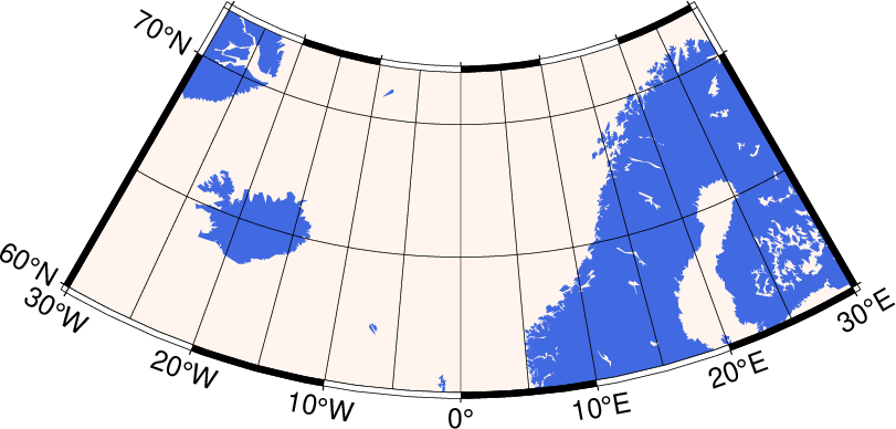
Polar stereographic conformal projection.

6.2.2.2. Rectangular stereographic map

As with Lambert’s azimuthal equal-area projection we have the option to use rectangular boundaries rather than the wedge-shape typically associated with polar projections. This choice is defined by selecting two points as corners in the rectangle and appending +r to the -R option. This command produces a map as presented in Figure Polar stereographic:

gmt begin GMT_stereographic_rect
	gmt set GMT_THEME cookbook
	gmt set MAP_ANNOT_OBLIQUE lon_horizontal,lat_horizontal,tick_extend,tick_normal
	gmt coast -R-25/59/70/72+r -JS10/90/11c -B20g -Dl -A250 -Gdarkbrown -Wthinnest -Slightgray
gmt end show

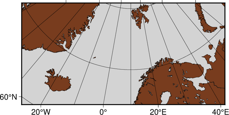
Polar stereographic conformal projection with rectangular borders.

6.2.2.3. General stereographic map

In terms of usage this projection is identical to the Lambert azimuthal equal-area projection. Thus, one can make both rectangular and hemispheric maps. Our example shows Australia using a projection pole at 130°E/30°S. The command used was

gmt begin GMT_stereographic_general
	gmt set GMT_THEME cookbook
	gmt set MAP_ANNOT_OBLIQUE separate
	gmt coast -R100/-42/160/-8+r -JS130/-30/12c -Bag -Dl -A500 -Ggreen -Slightblue -Wthinnest
gmt end show

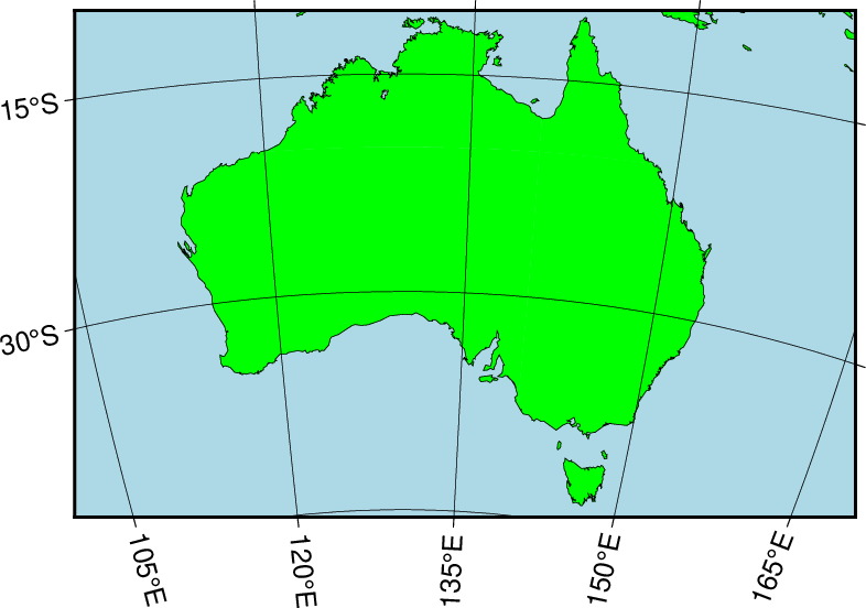
General stereographic conformal projection with rectangular borders.

By choosing 0/0 as the pole, we obtain the conformal stereonet presented next to its equal-area cousin in the Section Lambert Azimuthal Equal-Area (-Ja -JA) on the Lambert azimuthal equal-area projection (Figure Stereonets).

6.2.3. Perspective projection (-Jg -JG)

Syntax

-Jg|Glon0/lat0/scale|width[+aazimuth][+ttilt][+vvwidth/vheight][+wtwist][+zaltitude[r|R]|g]

Required Parameters

• The longitude (lon0) and latitude (lat0) of the projection center.

• The scale as 1:xxxxx or as radius/latitude where radius is distance on map in plot-units from projection center to a particular oblique latitude (with -Jg), or map width in plot-units (with -JG).

Optional Parameters

• The azimuth in degrees. This is the direction in which you are looking, measured clockwise from north [0].

• The tilt in degrees. This is the viewing angle relative to zenith. For example, a tilt of 0° is looking straight down, and 60° is looking from 30° above the horizon [0].

• The vwidth and vheight of the viewpoint in degrees. This number depends on whether you are looking with the naked eye (in which case the view is about 60° wide), or with binoculars, for example [unrestricted].

• The twist in degrees. This is the boresight rotation (clockwise) of the image [0].

• The altitude of the viewer above sea level in kilometers [infinity]. Alternatively, append R if giving the distance of the viewer from the center of the Earth in Earth radii, or r if giving the distance from the center of the Earth in kilometers. Finally, give altitude as g to compute and use the altitude for a geosynchronous orbit.

Description

The perspective projection imitates in 2 dimensions the 3-dimensional view of the earth from space. The implementation in GMT is very flexible, and thus requires many input variables.

Example

The imagined view of northwest Europe from a Space Shuttle at 230 km looking due east is thus accomplished by the following coast command (lon0=4; lat0=52; altitude=230 km; azimuth= 90°; tilt= 60°; twist= 180°; vwidth= vheight= 60°; and width = 12 cm):

gmt coast -Rg -JG4/52/12c+z230+a90+t60+w180+v60 -Bx2g2 -By1g1 -Ia -Di -Glightbrown -Wthinnest -Slightblue --GMT_THEME=cookbook --MAP_ANNOT_MIN_SPACING=0.6c -view GMT_perspective

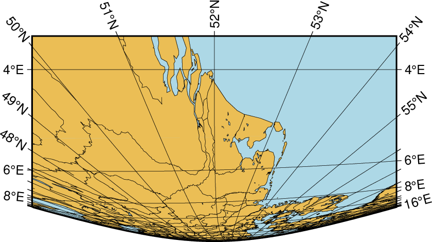
View from the Space Shuttle in Perspective projection.

6.2.4. Orthographic projection (-Jg -JG)

Syntax

-Jg|Glon0/lat0[/horizon]/scale|width

Parameters

• The longitude (lon0) and latitude (lat0) of the projection center.

• Optionally, the horizon, i.e., the number of degrees from the center to the edge (<=90) [default is 90].

• The scale as 1:xxxxx or as radius/latitude where radius is distance on map in plot-units from projection center to a particular oblique latitude (with -Jg), or map width in plot-units (with -JG).

Description

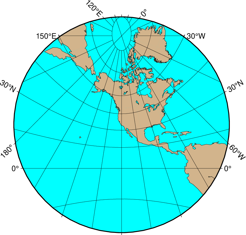
The orthographic azimuthal projection is a perspective projection from infinite distance. It is therefore often used to give the appearance of a globe viewed from outer space. As with Lambert’s equal-area and the stereographic projection, only one hemisphere can be viewed at any time. The projection is neither equal-area nor conformal, and much distortion is introduced near the edge of the hemisphere. The directions from the center of projection are true. The projection was known to the Egyptians and Greeks more than 2,000 years ago. Because it is mainly used for pictorial views at a small scale, only the spherical form is necessary.

Example

Our example of a perspective view centered on 75°W/40°N can therefore be generated by the following coast command:

gmt coast -Rg -JG-75/41/12c -Bg -Dc -A5000 -Gpink -Sthistle --GMT_THEME=cookbook -view GMT_orthographic

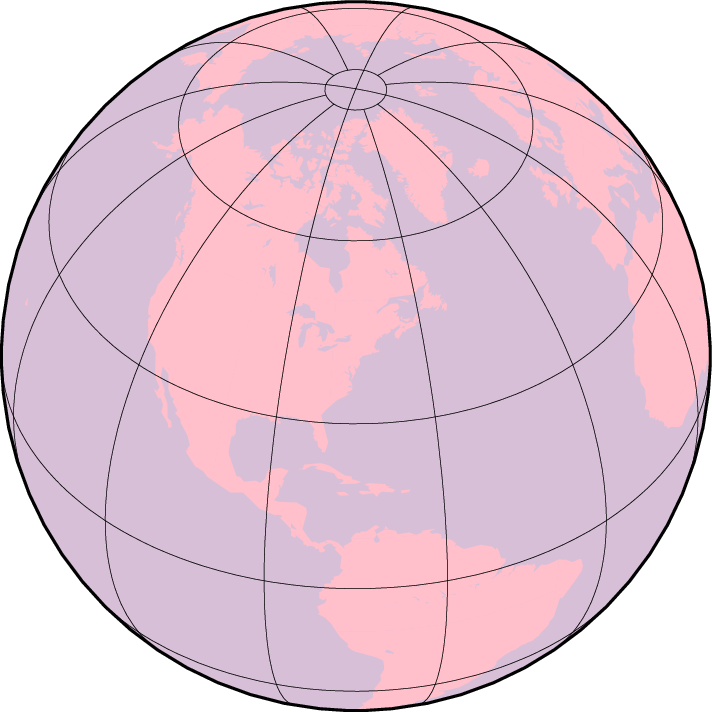
Hemisphere map using the Orthographic projection.

6.2.5. Azimuthal Equidistant projection (-Je -JE)

Syntax

-Je|Elon0/lat0[/horizon]scale|width

Parameters

• The longitude (lon0) and latitude (lat0) of the projection center.

• Optionally, the horizon, i.e., the number of degrees from the center to the edge (<=180) [default is 180].

• The scale as 1:xxxxx or as radius/latitude where radius is distance on map in plot-units from projection center to a particular oblique latitude (with -Je), or map width in plot-units (with -JE).

Description

The most noticeable feature of this azimuthal projection is the fact that distances measured from the center are true. Therefore, a circle about the projection center defines the locus of points that are equally far away from the plot origin. Furthermore, directions from the center are also true. The projection, in the polar aspect, is at least several centuries old. It is a useful projection for a global view of locations at various or identical distance from a given point (the map center).

Example

Our example of a global view centered on 100°W/40°N can therefore be generated by the following coast command. Note that the antipodal point is 180° away from the center, but in this projection this point plots as the entire map perimeter:

gmt coast -Rg -JE-100/40/12c -Bg -Dc -A10000 -Glightgray -Wthinnest --GMT_THEME=cookbook -view GMT_az_equidistant

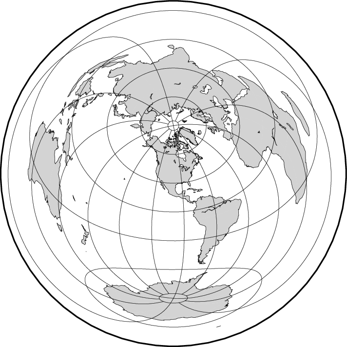
World map using the equidistant azimuthal projection.

6.2.6. Gnomonic projection (-Jf -JF)

Syntax

-Jf|Flon0/lat0[/horizon]scale|width

Parameters

• The longitude (lon0) and latitude (lat0) of the projection center.

• Optionally, the horizon, i.e., the number of degrees from the center to the edge (<90) [default is 60].

• The scale as 1:xxxxx or as radius/latitude where radius is distance on map in plot-units from projection center to a particular oblique latitude (with -Jf), or map width in plot-units (with -JF).

Description

The Gnomonic azimuthal projection is a perspective projection from the center onto a plane tangent to the surface. Its origin goes back to the old Greeks who used it for star maps almost 2500 years ago. The projection is neither equal-area nor conformal, and much distortion is introduced near the edge of the hemisphere; in fact, less than a hemisphere may be shown around a given center. The directions from the center of projection are true. Great circles project onto straight lines. Because it is mainly used for pictorial views at a small scale, only the spherical form is necessary.

Example

Using a horizon of 60, our example of this projection centered on 120°W/35°N can therefore be generated by the following coast command:

gmt coast -Rg -JF-120/35/60/12c -B30g15 -Dc -A10000 -Gtan -Scyan -Wthinnest --GMT_THEME=cookbook -view GMT_gnomonic

Gnomonic azimuthal projection.

6.3. Cylindrical projections

Cylindrical projections are easily recognized for their shape: maps are rectangular and meridians and parallels are straight lines crossing at right angles. But that is where similarities between the cylindrical projections supported by GMT (Mercator, transverse Mercator, universal transverse Mercator, oblique Mercator, Cassini, cylindrical equidistant, cylindrical equal-area, Miller, and cylindrical stereographic) stops. Each have a different way of spacing the meridians and parallels to obtain certain desirable cartographic properties.

6.3.1. Mercator projection (-Jm -JM)

Syntax

-Jm|M[lon0/[lat0/]]scale|width

Parameters

• Optionally, the central meridian (lon0) [default is the middle of the map].

• Optionally, the standard parallel for true scale (lat0) [default is the equator]. When supplied, the central meridian (lon0) must be supplied as well.

• The scale along the equator in plot-units/degree or as 1:xxxxx (with -Jm) or map width in plot-units (with -JM).

Description

Probably the most famous of the various map projections, the Mercator projection takes its name from the Flemish cartographer Gheert Cremer, better known as Gerardus Mercator, who presented it in 1569. The projection is a cylindrical and conformal, with no distortion along the equator. A major navigational feature of the projection is that a line of constant azimuth is straight. Such a line is called a rhumb line or loxodrome. Thus, to sail from one point to another one only had to connect the points with a straight line, determine the azimuth of the line, and keep this constant course for the entire voyage[21]. The Mercator projection has been used extensively for world maps in which the distortion towards the polar regions grows rather large, thus incorrectly giving the impression that, for example, Greenland is larger than South America. In reality, the latter is about eight times the size of Greenland. Also, the Former Soviet Union looks much bigger than Africa or South America. One may wonder whether this illusion has had any influence on U.S. foreign policy.

In the regular Mercator projection, the cylinder touches the globe along the equator. Other orientations like vertical and oblique give rise to the transverse Mercator and oblique Mercator projections, respectively. We will discuss these generalizations following the regular Mercator projection.

Example

A world map at a scale of 0.03 cm per degree, which will give a map 10.8-cm wide, can be obtained as follows:

gmt begin GMT_mercator
	gmt set GMT_THEME cookbook
	gmt set MAP_FRAME_TYPE fancy-rounded
	gmt coast -R0/360/-70/70 -Jm0.03c -Bxa60f15 -Bya30f15 -Dc -A5000 -Gred
gmt end show

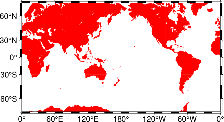
Simple Mercator map.

While this example is centered on the Dateline, one can easily choose another configuration with the -R option. For example, specify the region with -R-180/180/-70/70 to obtain a map centered on Greenwich.

6.3.2. Transverse Mercator projection (-Jt -JT)

Syntax

-Jt|Tlon0/[lat0/]scale|width

Parameters

• The central meridian (lon0).

• Optionally, the latitude of origin (lat0) [default is the equator].

• The scale along the equator in plot-units/degree or 1:xxxxx (with -Jt) or map width in plot-units (with -JT).

You can change the map scale factor via the PROJ_SCALE_FACTOR parameter [default is 1].

Description

The transverse Mercator was invented by Johann Heinrich Lambert in 1772. In this projection the cylinder touches a meridian along which there is no distortion. The distortion increases away from the central meridian and goes to infinity at 90° from center. The central meridian, each meridian 90° away from the center, and equator are straight lines; other parallels and meridians are complex curves.

Example

A transverse Mercator map of south-east Europe and the Middle East with 35°E as the central meridian can be obtained as follows:

gmt coast -R20/30/50/45+r -Jt35/0.5c -Bag -Dl -A250 -Glightbrown -Wthinnest -Sseashell --GMT_THEME=cookbook -view GMT_transverse_merc

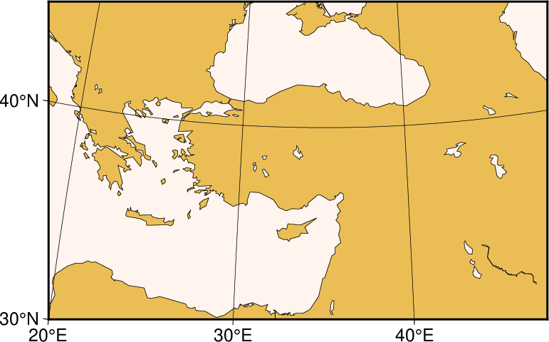
Rectangular Transverse Mercator map.

A global transverse Mercator map - the equivalent of the 360° Mercator map - can also be obtained as follows:

gmt coast -R0/360/-80/80 -JT330/-45/10c -Ba30g -BWSne -Dc -A2000 -Slightblue -G0 --MAP_ANNOT_OBLIQUE=lon_horizontal --GMT_THEME=cookbook -view GMT_TM

A global transverse Mercator map.

Note that when a world map is given (indicated by -R0/360/s/n), the arguments are interpreted to mean oblique degrees, i.e., the 360° range is understood to mean the extent of the plot along the central meridian, while the “south” and “north” values represent how far from the central longitude we want the plot to extend. These values correspond to latitudes in the regular Mercator projection and must therefore be less than 90.

6.3.3. Universal Transverse Mercator (UTM) projection (-Ju -JU)

Syntax

-Ju|Uzone/scale|width

Parameters

• UTM zone (A, B, 1–60, Y, Z). Use negative values for numerical zones in the southern hemisphere or append the latitude modifiers (C–H, J–N, P–X) to specify an exact UTM grid zone.

• The scale along the equator in plot-units/degree or as 1:xxxxx (with -Ju) or map width in plot-units (with -JU).

Description

A particular subset of the transverse Mercator is the Universal Transverse Mercator (UTM) which was adopted by the US Army for large-scale military maps. Here, the globe is divided into 60 zones between 84°S and 84°N, most of which are 6° wide. Each of these UTM zones have a unique central meridian. Furthermore, each zone is divided into latitude bands but these are not needed to specify the projection for most cases. See Figure Universal Transverse Mercator for all zone designations.

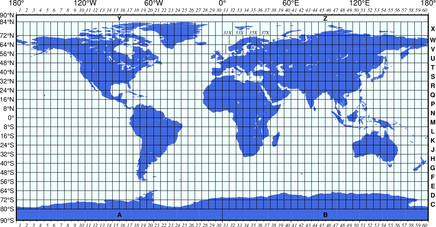
Universal Transverse Mercator zone layout.

Here is the source script for the figure above:

gmt begin GMT_utm_zones
gmt set GMT_THEME cookbook
gmt coast -Rd -JQ9i -Groyalblue -Sazure -Dl -A2000 -Bx60f6 -By0 -BwsNe --MAP_ANNOT_OFFSET_PRIMARY=0.15i
cat << EOF > tt.z.d
>  Do S pole zone
-180	-80
   0	-80
+180	-80
>
0	-90
0	-80
>  Do N pole zone
-180	84
   0	84
+180	84
>
0	90
0	84
EOF
gmt math -T-174/174/6 T 0 MUL = tt.x.d
echo '-90' > tt.L.d
let s=-80
rm -f tt.y.d
while [ $s -lt 72 ]; do
	echo $s >> tt.L.d
	n=$(($s+8))
	cat <<- EOF >> tt.z.d
	> Lat = $s
	-180	$s
	   0	$s
	+180	$s
	EOF
	if [ $s -eq 56 ]; then
		$AWK '{if ($1 == 6) {print 3} else {print $0}}' tt.x.d > tt.sp.d
	else
		cat tt.x.d > tt.sp.d
	fi
	$AWK '{printf "> \n%s\t%s\n%s\t%s\n", $1, "'$s'", $1, "'$n'"}' tt.sp.d >> tt.z.d
	gmt math -Q $s $n ADD 2 DIV = >> tt.y.d
	s=$n
done
echo $n >> tt.L.d
echo '84' >> tt.L.d
echo '90' >> tt.L.d
echo 78 >> tt.y.d
cat << EOF > tt.n.d
C
D
E
F
G
H
J
K
L
M
N
P
Q
R
S
T
U
V
W
X
EOF
n=84
cat << EOF >> tt.z.d
> Lat = $s
-180	$s
   0	$s
+180	$s
EOF
$AWK '{if ($1 <=0 || $1 >=42) print $0}' tt.x.d > tt.sp.d
cat << EOF >> tt.sp.d
9
21
33
EOF
$AWK '{printf "> \n%s\t%s\n%s\t%s\n", $1, "'$s'", $1, "'$n'"}' tt.sp.d >> tt.z.d
gmt plot -W0.5p -Ap tt.z.d
paste tt.y.d tt.n.d | $AWK '{printf "180 %s %s\n", $1, $2}' | gmt text -N -D0.1i/0 -F+f10p,Helvetica-Bold
gmt text -N -F+f10p,Helvetica-Bold << EOF
-90	-85	A
+90	-85	B
-90	87	Y
+90	87	Z
EOF
gmt math -T-180/174/6 T 3 ADD = | $AWK '{printf "%s -90 %d\n", $2, NR}' | gmt text -N -D0/-0.07i -F+f8p,Times-Italic+jCT
gmt math -T-180/174/6 T 3 ADD = | $AWK '{printf "%s 90 %d\n", $2, NR}' | gmt text -N -D0/0.07i -F+f8p,Times-Italic+jCB
gmt text -D0/0.025i -F+f8p,Times-Italic+jCB << EOF
4.5	72	31X
15	72	33X
27	72	35X
37.5	72	37X
EOF
$AWK '{if ($1 < 0) printf "-180 %s %s@.S\n", $1, -$1}' tt.L.d | gmt text -N -D-0.05i/0 -F+f10p+jRM
$AWK '{if ($1 > 0) printf "-180 %s %s@.N\n", $1,  $1}' tt.L.d | gmt text -N -D-0.05i/0 -F+f10p+jRM
echo "-180 0 0@." | gmt text -N -D-0.05i/0 -F+f10p+jRM
gmt end show

In order to minimize the distortion in any given zone, a scale factor of 0.9996 has been factored into the formulae (although a standard, you can change this with PROJ_SCALE_FACTOR). This makes the UTM projection a secant projection and not a tangent projection like the transverse Mercator above. The scale only varies by 1 part in 1,000 from true scale at equator. The ellipsoidal projection expressions are accurate for map areas that extend less than 10 away from the central meridian. For larger regions we use the conformal latitude in the general spherical formulae instead.

6.3.4. Oblique Mercator projection (-Jo -JO)

Option 1 Syntax

-Jo|O[a|A]lon0/lat0/azimuth/scale|width[+v]

Option 1 Parameters

• The longitude (lon0) and latitude (lat0) of projection center.

• The azimuth (azimuth) of the oblique equator.

• The scale in plot-units/degree or 1:xxxxx along oblique equator (with -Jo), or map width in plot-units (with -JO).

• Optionally, append +v to let the oblique Equator align with the y-axis [default is to align with the x-axis].

Option 2 Syntax

-Jo|O[b|B]lon0/lat0/lon1/lat1/scale|width[+v]

Option 2 Parameters

• The longitude (lon0) and latitude (lat0) of projection center.

• The longitude (lon1) and latitude (lat1) of a second point on oblique equator.

• The scale in plot-units/degree or 1:xxxxx along oblique equator (with -Jo), or map width in plot-units (with -JO).

• Optionally, append +v to let the oblique Equator align with the y-axis [default is to align with the x-axis].

Option 3 Syntax

-Jo|O[c|C]lon0/lat0/lonp/latp/scale|width[+v]

Option 3 Parameters

• The longitude (lon0) and latitude (lat0) of projection center.

• The longitude (lonp) and latitude (latp) of the projection pole.

• The scale in plot-units/degree or 1:xxxxx along oblique equator (with -Jo), or map width in plot-units (with -JO).

• Optionally, append +v to let the oblique Equator align with the y-axis [default is to align with the x-axis].

For all three definitions, the upper case A|B|C means we will allow projection poles in the southern hemisphere [default is to map any such poles to their antipodes in the northern hemisphere].

Description

Oblique configurations of the cylinder give rise to the oblique Mercator projection. It is particularly useful when mapping regions of large lateral extent in an oblique direction. Both parallels and meridians are complex curves. The projection was developed in the early 1900s by several workers.

Example

An oblique view of some Caribbean islands using Option 3 can be obtained as follows:

gmt begin GMT_obl_merc
    gmt set GMT_THEME cookbook
    gmt coast -R270/20/305/25+r -JOc280/25.5/22/69/12c -Bag -Di -A250 -Gburlywood -Wthinnest -TdjTR+f2+l -Sazure
gmt end show

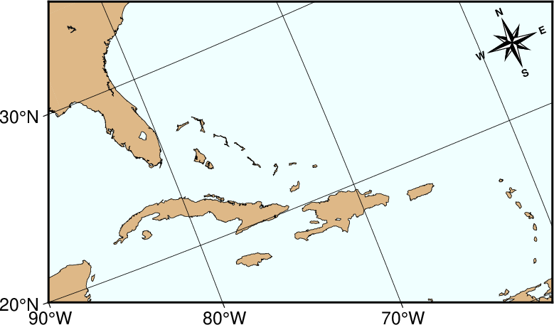
Oblique Mercator map using -JOc. We make it clear which direction is North by adding a star rose with the -Td option.

Note that we define our region using the rectangular system described earlier. If we do not append +r to the -R string then the information provided with the -R option is assumed to be oblique degrees about the projection center rather than the usual geographic coordinates. This interpretation is chosen since in general the parallels and meridians are not very suitable as map boundaries.

When working with oblique projections such as here, it is often much more convenient to specify the map domain in the projected coordinates relative to the map center. The figure below shows two views of New Zealand using the oblique Mercator projection that in both cases specifies the region using -R-1000/1000/-500/500+uk. The unit k means the following bounds are in projected km and we let GMT determine the geographic coordinates of the two diagonal corners internally.

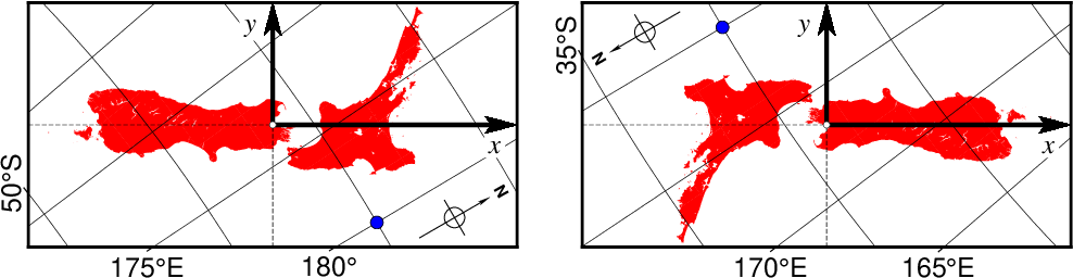
(left) Oblique view of New Zealand centered on its geographical center (Nelson) indicated by the white circle for an oblique Equator with azimuth 35. This resulted in the argument -JOa173:17:02E/41:16:15S/35/3i. The map is 2000 km by 1000 km and the Cartesian coordinate system in the projected units are indicated by the bold axes. The blue circle is the point (40S,180E) and it has projected coordinates (x = 426.2, y = -399.7). (right) Same dimensions but now specifying an azimuth of 215, yielding a projection pole in the southern hemisphere (hence we used -JOA to override the restriction, i.e., -JOA173:17:02E/41:16:15S/215/3i.) The projected coordinate system is still aligned as before but the Earth has been rotated 180 degrees. The blue point now has projected coordinates (x = -426.2, y = 399.7).

Here is the source script for the figure above:

gmt begin GMT_obl_nz
gmt set GMT_THEME cookbook
lon=173:17:02E
lat=41:16:15S
az=35
w=2000
h=1000
plon=180
plat=40S
w2=$(gmt math -Q $w 2 DIV =)
h2=$(gmt math -Q $h 2 DIV =)
R=-R-${w2}/$w2/-${h2}/${h2}+uk
gmt coast $R -JOA$lon/$lat/$az/3i -Ba5f5g5 -Gred -Dh -TdjBR+w0.5i+l --MAP_ANNOT_OBLIQUE=separate,lon_horizontal,lat_parallel --FORMAT_GEO_MAP=dddF
echo $plon $plat | gmt plot -Sc0.2c -Gblue -W0.25p
gmt plot -R0/3/0/1.5 -Jx1i -W0.25p,- << EOF
>
0	0.75
3	0.75
>
1.5	0
1.5	1.5
EOF
gmt plot -Sv0.2i+e+h0.5 -Gblack -W2p -N << EOF
1.5	0.75	0	1.5i
1.5	0.75	90	0.75i
EOF
echo 1.5 0.75 | gmt plot -Sc0.1c -Wfaint -Gwhite
gmt text -F+f12p,Times-Italic+j -Dj0.1i -Gwhite << EOF
3	0.75	TR	x
1.5	1.5	TR	y
EOF
az=215
gmt coast $R -JOA$lon/$lat/$az/3i -Ba5f5g5 -Gred -Dh -X3.4i -TdjTL+w0.5i+l --MAP_ANNOT_OBLIQUE=separate,lon_horizontal,lat_parallel --FORMAT_GEO_MAP=dddF
echo $plon $plat | gmt plot -Sc0.2c -Gblue -W0.25p
gmt plot -R0/3/0/1.5 -Jx1i -W0.25p,- << EOF
>
0	0.75
3	0.75
>
1.5	0
1.5	1.5
EOF
gmt plot -Sv0.2i+e+h0.5 -Gblack -W2p -N << EOF
1.5	0.75	0	1.5i
1.5	0.75	90	0.75i
EOF
echo 1.5 0.75 | gmt plot -Sc0.1c -Wfaint -Gwhite
gmt text -F+f12p,Times-Italic+j -Dj0.1i -Gwhite << EOF
3	0.75	TR	x
1.5	1.5	TR	y
EOF
gmt end show

The oblique Mercator projection will by default arrange the output so that the oblique Equator becomes the new horizontal, positive x-axis. For features with an orientation more north-south than east-west, it may be preferable to align the oblique Equator with the vertical, positive y-axis instead. This configuration is selected by appending +v to the -J projection option. The example below shows this behaviour.

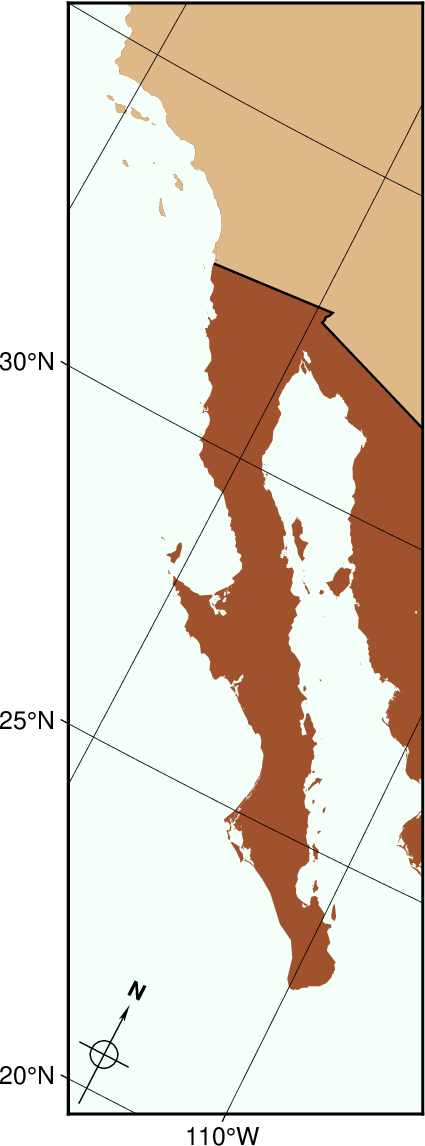
Oblique view of Baja California using the vertical oblique Equator modifier. This plot resulted from the argument -JOa120W/25N/-30/6c+v.

Here is the source script for the figure above:

gmt begin GMT_obl_baja
	gmt set GMT_THEME cookbook
	gmt set MAP_ANNOT_OBLIQUE lon_horizontal,lat_horizontal,tick_extend
	gmt coast -R122W/35N/107W/22N+r -JOa120W/25N/-30/6c+v -Gsienna -Ba5g5 -B+f -N1/1p -EUS+gburlywood -Smintcream -TdjBL+l
gmt end show

6.3.5. Cassini cylindrical projection (-Jc -JC)

Syntax

-Jc|Clon0/lat0/scale|width

Parameters

• The longitude (lon0) and latitude (lat0) of the central point.

• The scale in plot-units/degree or as 1:xxxxx (with -Jc) or map width in plot-units (with -JC).

Description

This cylindrical projection was developed in 1745 by César-François Cassini de Thury for the survey of France. It is occasionally called Cassini-Soldner since the latter provided the more accurate mathematical analysis that led to the development of the ellipsoidal formulae. The projection is neither conformal nor equal-area, and behaves as a compromise between the two end-members. The distortion is zero along the central meridian. It is best suited for mapping regions of north-south extent. The central meridian, each meridian 90° away, and equator are straight lines; all other meridians and parallels are complex curves.

Example

A detailed map of the island of Sardinia centered on the 8°45’E meridian using the Cassini projection can be obtained by as follows:

gmt coast -R7:30/38:30/10:30/41:30+r -JC8.75/40/6c -Bafg -LjBR+c40+w100+f+o0.4c/0.5c -Dh -Gspringgreen -Sazure -Wthinnest -Ia/thinner --GMT_THEME=cookbook --FONT_LABEL=10p -view GMT_cassini

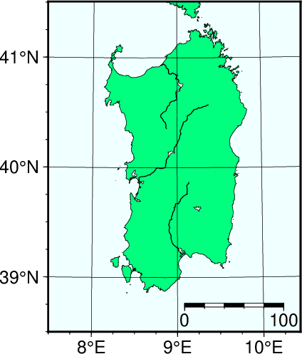
Cassini map over Sardinia.

As with the previous projections, the user can choose between a rectangular boundary (used here) or a geographical (WESN) boundary.

6.3.6. Cylindrical equidistant projection (-Jq -JQ)

Syntax

-Jq|Q[lon0/[lat0/]]scale|width

Parameters

• Optionally, the central meridian (lon0) [default is the middle of the map map].

• Optionally, the standard parallel (lat0) [default is the equator]. When supplied, the central meridian (lon0) must be supplied as well.

• The scale in plot-units/degree or as 1:xxxxx (with -Jq) or map width in plot-units (with -JQ).

Description

This simple cylindrical projection is really a linear scaling of longitudes and latitudes. The most common form is the Plate Carrée projection, where the scaling of longitudes and latitudes is the same. All meridians and parallels are straight lines.

Different relative scalings of longitudes and latitudes can be obtained by selecting a standard parallel different from the equator. Some selections for standard parallels have practical properties as shown in Table JQ.

Grafarend and Niermann, minimum linear distortion	61.7°
Ronald Miller Equirectangular	50.5°
Ronald Miller, minimum continental distortion	43.5°
Grafarend and Niermann	42°
Ronald Miller, minimum overall distortion	37.5°
Plate Carrée, Simple Cylindrical, Plain/Plane	0°

Example

A world map centered on the dateline using this projection can be obtained as follows:

gmt coast -Rg -JQ12c -B60f30g30 -Dc -A5000 -Gtan4 -Slightcyan --GMT_THEME=cookbook -view GMT_equi_cyl

World map using the Plate Carrée projection.

6.3.7. Cylindrical equal-area projections (-Jy -JY)

Syntax

-Jy|Y[lon0/[lat0/]]scale|width

Parameters

• Optionally, the central meridian (lon0) [default is the middle of the map].

• Optionally, the standard parallel (lat0) [default is the equator]. When supplied, the central meridian (lon0) must be supplied as well.

• The scale in plot-units/degree or as 1:xxxxx (with -Jy) or map width in plot-units (with -JY)

Description

This cylindrical projection is actually several projections, depending on what latitude is selected as the standard parallel. However, they are all equal area and hence non-conformal. All meridians and parallels are straight lines.

While you may choose any value for the standard parallel and obtain your own personal projection, there are seven choices of standard parallels that result in known (or named) projections. These are listed in Table JY.

Balthasart	50°
Gall	45°
Hobo-Dyer	37°30’ (= 37.5°)
Trystan Edwards	37°24’ (= 37.4°)
Caster	37°04’ (= 37.0666°)
Behrman	30°
Lambert	0°

Example

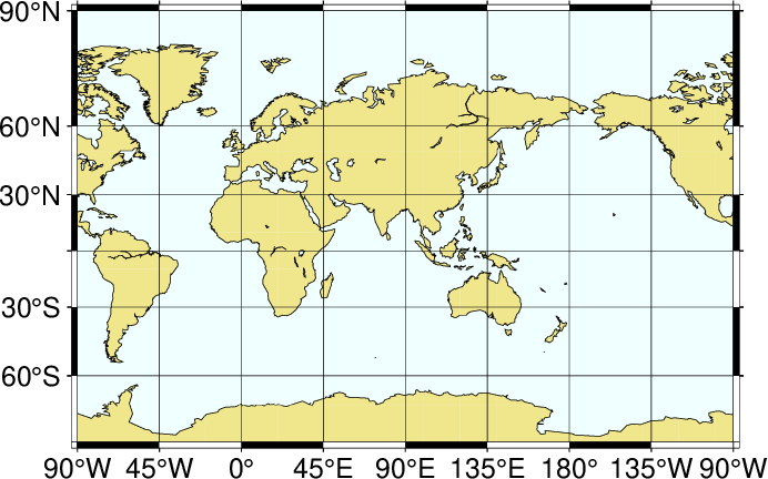
A world map centered on the 35°E meridian using the Behrman projection (Figure Behrman cylindrical projection) can be obtained as follows:

gmt coast -R-145/215/-90/90 -JY35/30/12c -B45g45 -Dc -A10000 -Sdodgerblue -Wthinnest --GMT_THEME=cookbook --MAP_FRAME_TYPE=fancy-rounded -view GMT_general_cyl

World map using the Behrman cylindrical equal-area projection.

As one can see there is considerable distortion at high latitudes since the poles map into lines.

6.3.8. Miller Cylindrical projection (-Jj -JJ)

Syntax

-Jj|J[lon0/]scale|width

Parameters

• Optionally, the central meridian (lon0) [default is the middle of the map].

• The scale in plot-units/degree or as 1:xxxxx (with -Jj) or map width in plot-units (with -JJ).

Description

This cylindrical projection, presented by Osborn Maitland Miller of the American Geographic Society in 1942, is neither equal nor conformal. All meridians and parallels are straight lines. The projection was designed to be a compromise between Mercator and other cylindrical projections. Specifically, Miller spaced the parallels by using Mercator’s formula with 0.8 times the actual latitude, thus avoiding the singular poles; the result was then divided by 0.8. There is only a spherical form for this projection.

Example

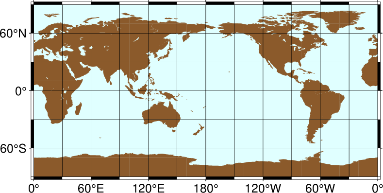
A world map centered on the 90°E meridian at a map scale of 1:400,000,000 (Figure Miller projection) can be obtained as follows:

gmt coast -R-90/270/-80/90 -Jj1:400000000 -Bx45g45 -By30g30 -Dc -A10000 -Gkhaki -Wthinnest -Sazure --GMT_THEME=cookbook -view GMT_miller

World map using the Miller cylindrical projection.

6.3.9. Cylindrical stereographic projections (-Jcyl_stere -JCyl_stere)

Syntax

-Jcyl_stere|Cyl_stere/[lon0/[lat0/]]scale|width

Parameters

• Optionally, the central meridian (lon0) [default is the middle of the map].

• Optionally, the standard parallel (lat0) [default is the Equator]. When used, central meridian (lon0) needs to be given as well.

• The scale in plot-units/degree or as 1:xxxxx (with -Jcyl_stere) or map width in plot-units (with -JCyl_stere).

Description

The cylindrical stereographic projections are certainly not as notable as other cylindrical projections, but are still used because of their relative simplicity and their ability to overcome some of the downsides of other cylindrical projections, like extreme distortions of the higher latitudes. The stereographic projections are perspective projections, projecting the sphere onto a cylinder in the direction of the antipodal point on the equator. The cylinder crosses the sphere at two standard parallels, equidistant from the equator.

Some of the selections of the standard parallel are named for the cartographer or publication that popularized the projection (Table JCylstere).

Miller’s modified Gall	66.159467°
Kamenetskiy’s First	55°
Gall’s stereographic	45°
Bolshoi Sovietskii Atlas Mira or Kamenetskiy’s Second	30°
Braun’s cylindrical	0°

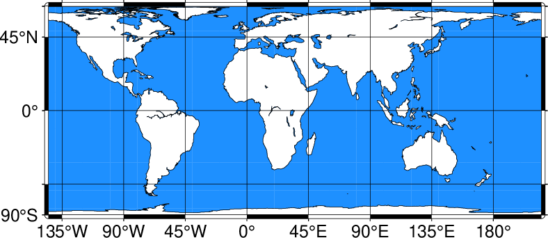
Example

A map of the world, centered on the Greenwich meridian, using the Gall’s stereographic projection (standard parallel is 45°, Figure Gall’s stereographic projection), can be obtained as follows:

gmt begin GMT_gall_stereo
	gmt set GMT_THEME cookbook
	gmt set FORMAT_GEO_MAP dddA
	gmt coast -R-180/180/-60/80 -JCyl_stere/0/45/12c -Bxa60f30g30 -Bya30g30 -Dc -A5000 -Wblack -Gseashell4 -Santiquewhite1
gmt end show

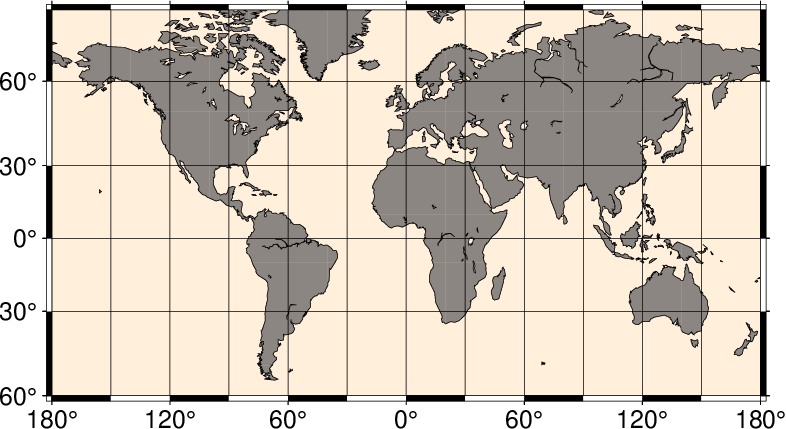
World map using Gall’s stereographic projection.

6.4. Miscellaneous projections

GMT supports eight common projections for global presentation of data or models. These are the Hammer, Mollweide, Winkel Tripel, Robinson, Eckert IV and VI, Sinusoidal, and Van der Grinten projections. Due to the small scale used for global maps these projections all use the spherical approximation rather than more elaborate elliptical formulae.

In all cases, the specification of the central meridian can be skipped. The default is the middle of the longitude range of the plot, specified by the (-R) option.

6.4.1. Hammer projection (-Jh -JH)

Syntax

-Jh|H[lon0/]scale|width

Parameters

• The central meridian (lon0) [default is the middle of the map].

• The scale along equator in plot-units/degree or as 1:xxxxx (with -Jh) or map width in plot-units (with -JH).

Description

The equal-area Hammer projection, first presented by the German mathematician Ernst von Hammer in 1892, is also known as Hammer-Aitoff (the Aitoff projection looks similar, but is not equal-area). The border is an ellipse, equator and central meridian are straight lines, while other parallels and meridians are complex curves.

Example

A view of the Pacific ocean using the Dateline as central meridian can be generated thus:

gmt coast -Rg -JH12c -Bg -Dc -A10000 -Gblack -Scornsilk --GMT_THEME=cookbook -view GMT_hammer

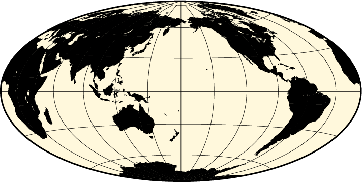
World map using the Hammer projection.

6.4.2. Mollweide projection (-Jw -JW)

Syntax

-Jw|W[lon0/]scale|width

Parameters

• The central meridian (lon0) [default is the middle of the map].

• The scale along equator in plot-units/degree or as 1:xxxxx (with -Jw) or map width in plot-units (with -JW).

Description

This pseudo-cylindrical, equal-area projection was developed by the German mathematician and astronomer Karl Brandan Mollweide in 1805. Parallels are unequally spaced straight lines with the meridians being equally spaced elliptical arcs. The scale is only true along latitudes 40°44’ north and south. The projection is used mainly for global maps showing data distributions. It is occasionally referenced under the name homalographic projection.

Example

An example centered on Greenwich can be generated thus:

gmt coast -Rd -JW12c -Bg -Dc -A10000 -Gtomato1 -Sskyblue --GMT_THEME=cookbook -view GMT_mollweide

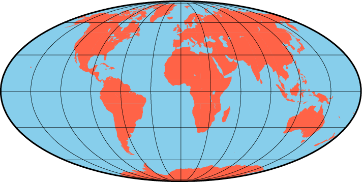
World map using the Mollweide projection.

6.4.3. Winkel Tripel projection (-Jr -JR)

Syntax

-Jr|R[lon0/]scale|width

Parameters

• The central meridian (lon0) [default is the middle of the map].

• The scale along equator in plot-units/degree or as 1:xxxxx (with -Jr) or map width in plot-units (with -JR).

Description

In 1921, the German mathematician Oswald Winkel created a projection that was to strike a compromise between the properties of three elements (area, angle and distance). The German word “tripel” refers to this junction of where each of these elements are least distorted when plotting global maps. The projection was popularized when Bartholomew and Son started to use it in its world-renowned “The Times Atlas of the World” in the mid-20th century. In 1998, the National Geographic Society made the Winkel Tripel as its map projection of choice for global maps.

Naturally, this projection is neither conformal, nor equal-area. Central meridian and equator are straight lines; other parallels and meridians are curved. The projection is obtained by averaging the coordinates of the Equidistant Cylindrical and Aitoff (not Hammer-Aitoff) projections. The poles map into straight lines 0.4 times the length of equator.

Example

Centered on Greenwich, the example in Figure Winkel Tripel projection was created by this command:

gmt coast -Rd -JR12c -Bg -Dc -A10000 -Gburlywood4 -Swheat1 --GMT_THEME=cookbook -view GMT_winkel

World map using the Winkel Tripel projection.

6.4.4. Robinson projection (-Jn -JN)

Syntax

-Jn|N[lon0/]scale|width

Parameters

• The central meridian (lon0) [default is the middle of the map].

• The scale along equator in plot-units/degree or as 1:xxxxx (with -Jn) or map width in plot-units (with -JN).

Description

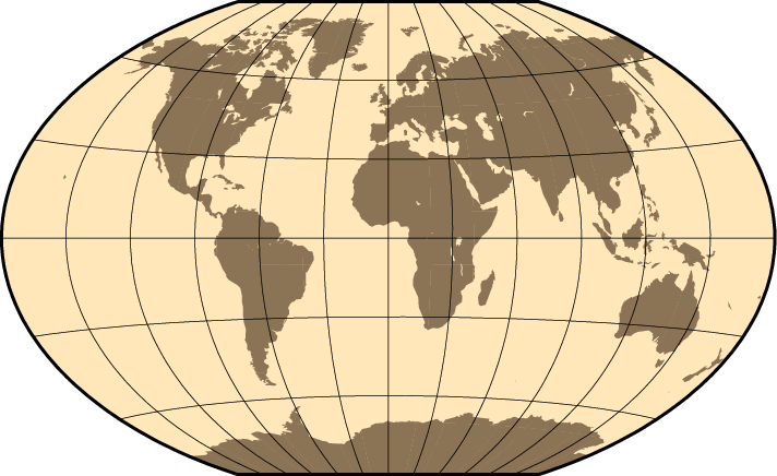
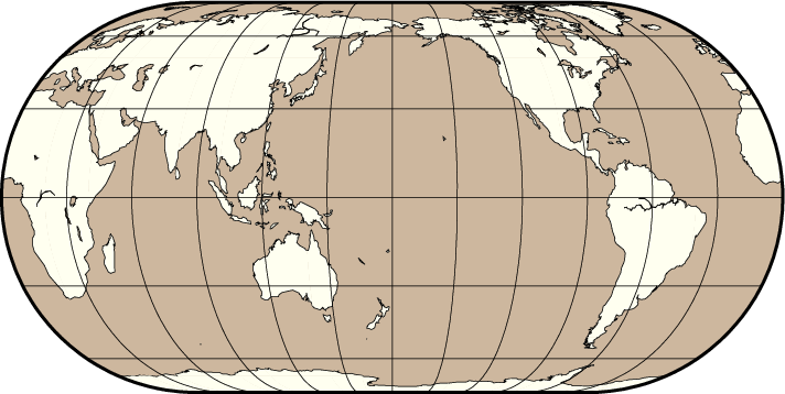
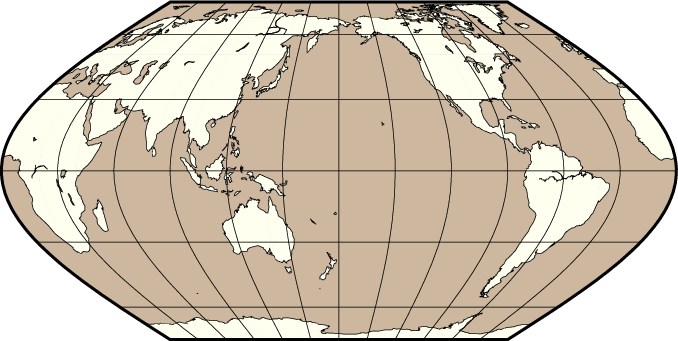
The Robinson projection, presented by the American geographer and cartographer Arthur H. Robinson in 1963, is a modified cylindrical projection that is neither conformal nor equal-area. Central meridian and all parallels are straight lines; other meridians are curved. It uses lookup tables rather than analytic expressions to make the world map “look” right[22]. The scale is true along latitudes 38. The projection was originally developed for use by Rand McNally and is currently used by the National Geographic Society.

Example

Again centered on Greenwich, the example below was created by this command:

gmt coast -Rd -JN12c -Bg -Dc -A10000 -Ggoldenrod -Ssnow2 --GMT_THEME=cookbook -view GMT_robinson

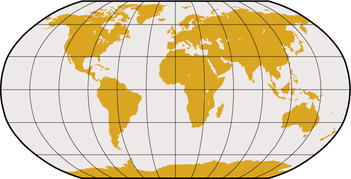
World map using the Robinson projection.

6.4.5. Eckert IV and VI projection (-Jk -JK)

Syntax

-Jk|Kf[lon0/]scale|width (Eckert IV) -Jk|K[s][lon0/]scale|width (Eckert VI)

Parameters

• The central meridian (lon0) [default is the middle of the map].

• The scale along equator in plot-units/degree or as 1:xxxxx (with -Jk) or map width in plot-units (with -JK).

Description

The Eckert IV and VI projections, presented by the German cartographer Max Eckert-Greiffendorff in 1906, are pseudo-cylindrical equal-area projections. Central meridian and all parallels are straight lines; other meridians are equally spaced elliptical arcs (IV) or sinusoids (VI). The scale is true along latitudes 40°30’ (IV) and 49°16’ (VI). Their main use is in thematic world maps. To select Eckert IV you must use -JKf (f for “four”) while Eckert VI is selected with -JKs (s for “six”). If no modifier is given it defaults to Eckert VI.

Examples

Centered on the Dateline, the Eckert IV example below was created by this command:

gmt coast -Rg -JKf12c -Bg -Dc -A10000 -Wthinnest -Givory -Sbisque3 --GMT_THEME=cookbook -view GMT_eckert4

World map using the Eckert IV projection.

The same script, with s instead of f, yields the Eckert VI map:

World map using the Eckert VI projection.

Here is the source script for the figure above:

gmt begin GMT_eckert6
	gmt set GMT_THEME cookbook
	gmt coast -Rg -JKs4.5i -Bg -Dc -A10000 -Wthinnest -Givory -Sbisque3
gmt end show

6.4.6. Sinusoidal projection (-Ji -JI)

Syntax

-Ji|I[lon0/]scale|width

Parameters

• The central meridian (lon0) [default is the middle of the map].

• The scale along equator in plot-units/degree or as 1:xxxxx (with -Ji) or map width in plot-units (with -JI).

Description

The sinusoidal projection is one of the oldest known projections, is equal-area, and has been used since the mid-16th century. It has also been called the “Equal-area Mercator” projection. The central meridian is a straight line; all other meridians are sinusoidal curves. Parallels are all equally spaced straight lines, with scale being true along all parallels (and central meridian).

Examples

A simple world map using the sinusoidal projection is therefore obtained by

gmt coast -Rd -JI12c -Bg -Dc -A10000 -Gcoral4 -Sazure3 --GMT_THEME=cookbook -view GMT_sinusoidal

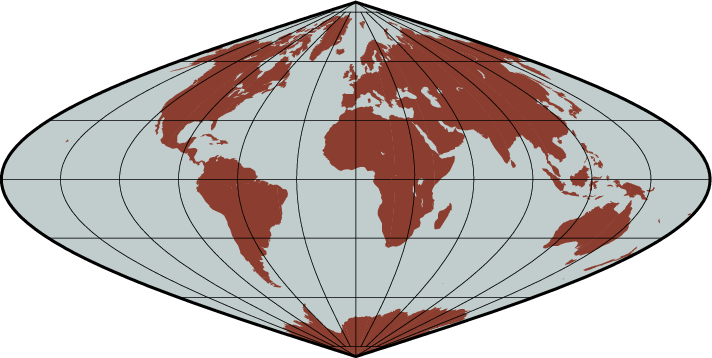
World map using the Sinusoidal projection.

To reduce distortion of shape the interrupted sinusoidal projection was introduced in 1927. Here, three symmetrical segments are used to cover the entire world. Traditionally, the interruptions are at 160°W, 20°W, and 60°E. To make the interrupted map we must call coast for each segment and superpose the results. To produce an interrupted world map (with the traditional boundaries just mentioned) that is 14.4 cm wide we use the scale 14.4/360 = 0.04 and offset the subsequent plots horizontally by their widths (140\(\cdot\)0.04 and 80\(\cdot\)0.04):

gmt begin GMT_sinus_int
	gmt set GMT_THEME cookbook
	gmt coast -R200/340/-90/90 -Ji0.04c -Bg -A10000 -Dc -Gdarkred -Sazure
	gmt coast -R-20/60/-90/90 -Bg -Dc -A10000 -Gdarkgreen -Sazure -X5.6c
	gmt coast -R60/200/-90/90 -Bg -Dc -A10000 -Gdarkblue -Sazure -X3.2c
gmt end show

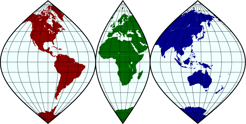
World map using the Interrupted Sinusoidal projection.

The usefulness of the interrupted sinusoidal projection is basically limited to display of global, discontinuous data distributions like hydrocarbon and mineral resources, etc.

6.4.7. Van der Grinten projection (-Jv -JV)

Syntax

-Jv|V[lon0/]scale|width

Parameters

• The central meridian (lon0) [default is the middle of the map].

• The scale along equator in plot-units/degree or as 1:xxxxx (with -Jv) or map width in plot-units (with -JV).

Description

The Van der Grinten projection, presented by Alphons J. van der Grinten in 1904, is neither equal-area nor conformal. Central meridian and Equator are straight lines; other meridians are arcs of circles. The scale is true along the Equator only. Its main use is to show the entire world enclosed in a circle.

Example

Centered on the Dateline, the example below was created by this command:

gmt coast -Rg -JV10c -Bg -Dc -Glightgray -Scornsilk -A10000 -Wthinnest --GMT_THEME=cookbook -view GMT_grinten

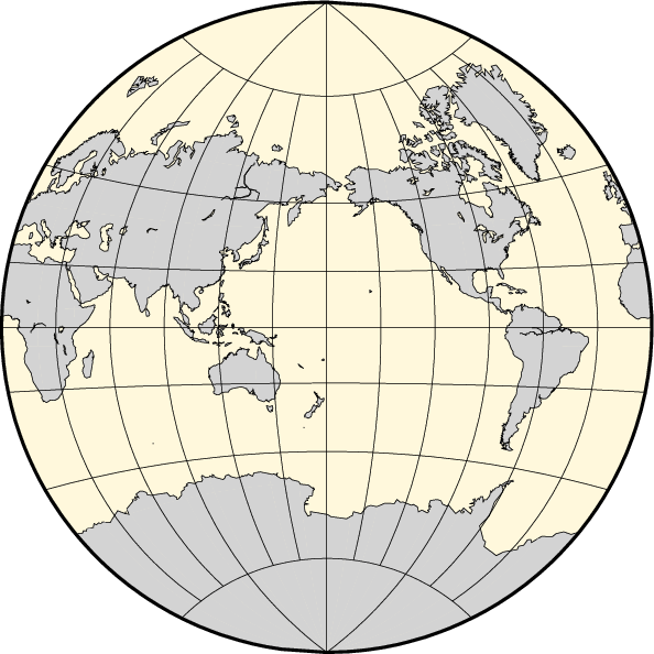
World map using the Van der Grinten projection.

6.5. Footnotes

[20]

Snyder, J. P., 1987, Map Projections A Working Manual, U.S. Geological Survey Prof. Paper 1395.

[21]

This is, however, not the shortest distance. It is given by the great circle connecting the two points.

[22]

Robinson provided a table of y-coordinates for latitudes every 5. To project values for intermediate latitudes one must interpolate the table. Different interpolants may result in slightly different maps. GMT uses the interpolant selected by the parameter GMT_INTERPOLANT in the file.