8. GMT File Formats
8.1. Table data
These files have N records which have M fields each. All programs that handle tables can read multicolumn files. GMT can read both ASCII, native binary, netCDF table data, and ESRI shapefiles (which we convert to GMT/OGR format via GDAL’s ogr2ogr tool under the hood).
8.1.1. ASCII tables
8.1.1.1. Optional file header records
The first data record may be preceded by one or more header records. Any records that begins with ‘#’ is considered a header or comment line and are always processed correctly. If your data file has leading header records that do not start with ‘#’ then you must make sure to use the -h option and set the parameter IO_N_HEADER_RECS in the gmt.conf file (GMT default is one header record if -h is given; you may also use -hnrecs directly). Alternatively, you can override the header record marker ‘#’ by modifying the IO_HEADER_MARKER default setting. Fields within a record must be separated by spaces, tabs, commas, or semi-colons. Each field can be an integer or floating-point number or a geographic coordinate string using the [±]dd[:mm[:ss[.xx…]]][W|E|S|N|w|e|s|n] format. Thus, 12:30:44.5W, 17.5S, 1:00:05, and 200:45E are all valid input strings. GMT is expected to handle most CVS (Comma-Separated Values) files, including numbers given in double quotes. On output, fields will be separated by the character given by the parameter IO_COL_SEPARATOR, which by default is a TAB.
8.1.1.2. Optional segment header records
When dealing with time- or (x,y)-series it is usually convenient to have each profile in separate files. However, this may sometimes prove impractical due to large numbers of profiles. An example is files of digitized lineations where the number of individual features may range into the thousands. One file per feature would in this case be unreasonable and furthermore clog up the directory. GMT provides a mechanism for keeping more than one profile in a file. Such files are called multiple segment files and are identical to the ones just outlined except that they have segment headers interspersed with data records that signal the start of a new segment. The segment headers may be of any format, but all must have the same character in the first column. The unique character is by default ‘>’, but you can override that by modifying the IO_SEGMENT_MARKER default setting. Programs can examine the segment headers to see if they contain -D for a distance value, -W and -G options for specifying pen and fill attributes for individual segments, -Z to change color via a CPT, -L for label specifications, or -T for general-purpose text descriptions. These settings (and occasionally others) will override the corresponding command line options. GMT also provides for two special values for IO_SEGMENT_MARKER that can make interoperability with other software packages easier. Choose the marker B to have blank lines recognized as segment breaks, or use N to have data records whose fields equal NaN mean segment breaks (e.g., as used by Matlab or Octave). When these markers are used then no other segment header will be considered. Note that IO_SEGMENT_MARKER can be set differently for input and output. Finally, if a segment represents a closed polygon that is a hole inside another polygon you indicate this by including -Ph in the segment header. This setting will be read and processed if converting a file to the OGR format.
8.1.2. Binary tables
GMT programs also support native binary tables to speed up input-output for i/o-intensive tasks like gridding and preprocessing. This is discussed in more detail in section Map frame and axes annotations: The -B option.
8.1.3. NetCDF tables
More and more programs are now producing binary data in the netCDF format, and so GMT programs started to support tabular netCDF data (files containing one or more 1-dimensional arrays) starting with GMT version 4.3.0. Because of the meta data contained in those files, reading them is much less complex than reading native binary tables, and even than ASCII tables. GMT programs will read as many 1-dimensional columns as are needed by the program, starting with the first 1-dimensional it can find in the file. To specifically specify which variables are to be read, append the suffix ?var1/var2/… to the netCDF file name or add the option -bicvar1/var2/…, where var1, var2, etc.are the names of the variables to be processed. The latter option is particularly practical when more than one file is read: the -bic option will apply to all files. Currently, GMT only reads, but does not write, netCDF tabular data.
8.2. Grid files
GMT allows numerous grid formats to be read. In addition to the default
netCDF format it can use binary floating points, short integers, bytes, and
bits, as well as 8-bit Sun raster files (colormap ignored). Additional
formats may be used by supplying read/write functions and linking these with
the GMT libraries. The source file gmt_customio.c has the information
that programmers will need to augment GMT to read custom grid files. See
Section Grid file format specifications for more information.
8.2.1. NetCDF files
By default, GMT stores 2-D grids as COARDS-compliant netCDF files. COARDS (which stands for Cooperative Ocean/Atmosphere Research Data Service) is a convention used by many agencies distributing gridded data for ocean and atmosphere research. Sticking to this convention allows GMT to read gridded data provided by other institutes and other programs. Conversely, other general domain programs will be able to read grids created by GMT. COARDS is a subset of a more extensive convention for netCDF data called CF-1.5 (Climate and Forecast, version 1.5). Hence, GMT grids are also automatically CF-1.5-compliant. However, since CF-1.5 has more general application than COARDS, not all CF-1.5 compliant netCDF files can be read by GMT.
The netCDF grid file in GMT has several attributes (See Table netcdf-format) to describe the content. The routine that deals with netCDF grid files is sufficiently flexible so that grid files slightly deviating from the standards used by GMT can also be read.
| Attribute | Description |
|---|---|
| Global attributes | |
| Conventions | COARDS, CF-1.5 (optional) |
| title | Title (optional) |
| source | How file was created (optional) |
| node_offset | 0 for gridline node registration (default), 1 for pixel registration |
| x- and y-variable attributes | |
| long_name | Coordinate name (e.g., “Longitude” and “Latitude”) |
| units | Unit of the coordinate (e.g., “degrees_east” and “degrees_north”) |
| actual range (or valid range) | Minimum and maximum x and y of region; if absent the first and last x- and y-values are queried |
| z-variable attributes | |
| long_name | Name of the variable (default: “z”) |
| units | Unit of the variable |
| scale_factor | Factor to multiply z with (default: 1) |
| add_offset | Offset to add to scaled z (default: 0) |
| actual_range | Minimum and maximum z (in unpacked units, optional) and z |
| _FillValue (or missing_value) | Value associated with missing or invalid data points; if absent an appropriate default value is assumed, depending on data type. |
By default, the first 2-dimensional variable in a netCDF file will be read as the z variable and the coordinate axes x and y will be determined from the dimensions of the z variable. GMT will recognize whether the y (latitude) variable increases or decreases. Both forms of data storage are handled appropriately.
For more information on the use of COARDS-compliant netCDF files, and on how to load multi-dimensional grids, read Section Modifiers for COARDS-compliant netCDF files.
8.2.2. Chunking and compression with netCDF
GMT supports reading and writing of netCDF-4 files since release 5.0. For performance reasons with ever-increasing grid sizes, the default output format of GMT is netCDF-4 with chunking enabled for grids with more than 16384 cells. Chunking means that the data are not stored sequentially in rows along latitude but rather split up into tiles. Figure Grid split into 3 by 3 chunks illustrates the layout in a chunked netCDF file. To access a subset of the data (e.g., the four blue tiles in the lower left), netCDF only reads those tiles (“chunks”) instead of extracting data from long rows.
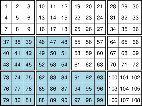
Grid split into 3 by 3 chunks
Gridded datasets in the earth sciences usually exhibit a strong spatial dependence (e.g. topography, potential fields, illustrated by blue and white cells in Figure Grid split into 3 by 3 chunks) and deflation can greatly reduce the file size and hence the file access time (deflating/inflating is faster than hard disk I/O). It is therefore convenient to deflate grids with spatial dependence (levels 1–3 give the best speed/size-tradeoff).
You may control the size of the chunks of data and compression with the configuration parameters IO_NC4_CHUNK_SIZE and IO_NC 4_DEFLATION_LEVEL as specified in gmt.conf and you can check the netCDF format with grdinfo.
Classic netCDF files were the de facto standard until netCDF 4.0 was released in 2008. Most programs supporting netCDF by now are using the netCDF-4 library and are thus capable of reading netCDF files generated with GMT 5, this includes official GMT releases since revision 4.5.8. In rare occasions, when you have to load netCDF files with old software, you may be forced to export your grids in the old classic format. This can be achieved by setting IO_NC4_CHUNK_SIZE to classic.
Further reading:
8.2.3. Gridline and Pixel node registration
Scanline format means that the data are stored in rows (y = constant) going from the “top” (\(y = y_{max}\) (north)) to the “bottom” (\(y = y_{min}\) (south)). Data within each row are ordered from “left” (\(x = x_{min}\) (west)) to “right” (\(x = x_{max}\) (east)). The registration signals how the nodes are laid out. The grid is always defined as the intersections of all x ( \(x = x_{min}, x_{min} + x_{inc}, x_{min} + 2 \cdot x_{inc}, \ldots, x_{max}\) ) and y ( \(y = y_{min}, y_{min} + y_{inc}, y_{min} + 2 \cdot y_{inc}, \ldots, y_{max}\) ) lines. The two scenarios differ as to which area each data point represents. The default node registration in GMT is gridline node registration. Most programs can handle both types, and for some programs like grdimage a pixel registered file makes more sense. Utility programs like grdsample and grdproject will allow you to convert from one format to the other; grdedit can make changes to the grid header and convert a pixel- to a gridline-registered grid, or vice versa. The grid registration is determined by the common GMT -r option (see Section Grid registration: The -r option).
8.2.4. Boundary Conditions for operations on grids
GMT has the option to specify boundary conditions in some programs that operate on grids (e.g., grdsample, grdgradient, grdtrack, nearneighbor, and grdview, to name a few. The desired condition can be set with the common GMT option -n; see Section Grid interpolation parameters: The -n option. The boundary conditions come into play when interpolating or computing derivatives near the limits of the region covered by the grid. The default boundary conditions used are those which are “natural” for the boundary of a minimum curvature interpolating surface. If the user knows that the data are periodic in x (and/or y), or that the data cover a sphere with x,y representing longitude,latitude, then there are better choices for the boundary conditions. Periodic conditions on x (and/or y) are chosen by specifying x (and/or y) as the boundary condition flags; global spherical cases are specified using the g (geographical) flag. Behavior of these conditions is as follows:
- Periodic
- conditions on x indicate that the data are periodic in the distance (\(x_{max} - x_{min}\)) and thus repeat values after every \(N = (x_{max} - x_{min})/x_{inc}\). Note that this implies that in a grid-registered file the values in the first and last columns are equal, since these are located at \(x = x_{min}\) and \(x = x_{max}\), and there are N + 1 columns in the file. This is not the case in a pixel-registered file, where there are only N and the first and last columns are located at \(x_{min} + x_{inc}/2\) and \(x_{max} - x_{inc}/2\). If y is periodic all the same holds for y.
- Geographical
conditions indicate the following:
- If \((x_{max} - x_{min}) \geq 360\) and also 180 modulo \(x_{inc} = 0\) then a periodic condition is used on x with a period of 360; else a default condition is used on the x boundaries.
- If condition 1 is true and also \(y_{max} = 90\) then a “north pole condition” is used at \(y_{max}\), else a default condition is used there.
- If condition 1 is true and also \(y_{min} = -90\) then a “south pole condition” is used at \(y_{min}\), else a default condition is used there.
“Pole conditions” use a 180º phase-shift of the data, requiring 180 modulo \(x_{inc} = 0\).
- Default
boundary conditions are
\[\nabla^2 f = \frac{\partial}{\partial n} \nabla^2 f = 0\]on the boundary, where \(f(x, y)\) is represented by the values in the grid file, and \(\partial/\partial n\) is the derivative in the direction normal to a boundary, and
\[\nabla^2 = \left(\frac{\partial^2}{\partial x^2} + \frac{\partial^2}{\partial y^2}\right)\]is the two-dimensional Laplacian operator.
8.2.5. Native binary grid files
The old-style native grid file format that was common in earlier version of GMT is still supported, although the use of netCDF files is strongly recommended. The file starts with a header of 892 bytes containing a number of attributes defining the content. The grdedit utility program will allow you to edit parts of the header of an existing grid file. The attributes listed in Table grdheader are contained within the header record in the order given (except the z-array which is not part of the header structure, but makes up the rest of the file). As this header was designed long before 64-bit architectures became available, the jump from the first three integers to the subsequent doubles in the structure does not occur on a 16-byte alignment. While GMT handles the reading of these structures correctly, enterprising programmers must take care to read this header correctly (see our code for details).
| Parameter | Description |
|---|---|
| int n_columns | Number of nodes in the x-dimension |
| int n_rows | Number of nodes in the y-dimension |
| int registration | 0 for grid line registration, 1 for pixel registration |
| double x_min | Minimum x-value of region |
| double x_max | Maximum x-value of region |
| double y_min | Minimum y-value of region |
| double y_max | Maximum y-value of region |
| double z_min | Minimum z-value in data set |
| double z_max | Maximum z-value in data set |
| double x_inc | Node spacing in x-dimension |
| double y_inc | Node spacing in y-dimension |
| double z_scale_factor | Factor to multiply z-values after read |
| double z_add_offset | Offset to add to scaled z-values |
| char x_units[80] | Units of the x-dimension |
| char y_units[80] | Units of the y-dimension |
| char z_units[80] | Units of the z-dimension |
| char title[80] | Descriptive title of the data set |
| char command[320] | Command line that produced the grid file |
| char remark[160] | Any additional comments |
| TYPE z[n_columns*n_rows] | 1-D array with z-values in scanline format |
8.3. Sun raster files
The Sun raster file format consists of a header followed by a series of unsigned 1-byte integers that represents the bit-pattern. Bits are scanline oriented, and each row must contain an even number of bytes. The predefined 1-bit patterns in GMT have dimensions of 64 by 64, but other sizes will be accepted when using the -Gp|P option. The Sun header structure is outline in Table sunheader.
| Parameter | Description |
|---|---|
| int ras_magic | Magic number |
| int ras_width | Width (pixels) of image |
| int ras_height | Height (pixels) of image |
| int ras_depth | Depth (1, 8, 24, 32 bits) of pixel |
| int ras_length | Length (bytes) of image |
| int ras_type | Type of file; see RT_ below |
| int ras_maptype | Type of colormap; see RMT_ below |
| int ras_maplength | Length (bytes) of following map |
After the header, the color map (if ras_maptype is not RMT_NONE) follows for ras_maplength bytes, followed by an image of ras_length bytes. Some related definitions are given in Table sundef.
| Macro name | Description |
|---|---|
| RAS_MAGIC | 0x59a66a95 |
| RT_STANDARD | 1 (Raw pixrect image in 68000 byte order) |
| RT_BYTE_ENCODED | 2 (Run-length compression of bytes) |
| RT_FORMAT_RGB | 3 ([X]RGB instead of [X]BGR) |
| RMT_NONE | 0 (ras_maplength is expected to be 0) |
| RMT_EQUAL_RGB | 1 (red[ras_maplength/3],green[],blue[]) |
Numerous public-domain programs exist, such as xv and convert (in the GraphicsMagick or ImageMagick package), that will translate between various raster file formats such as tiff, gif, jpeg, and Sun raster. Raster patterns may be created with GMT plotting tools by generating PostScript plots that can be rasterized by ghostscript and translated into the right raster format.