4. Standardized command line options¶

Most of the programs take many of the same arguments such as those related to setting the data region, the map projection, etc. The switches in Table switches have the same meaning in all the programs (although some programs may not use all of them). These options will be described here as well as in the manual pages, as is vital that you understand how to use these options. We will present these options in order of importance (some are used a lot more than others).


-B	Define tick marks, annotations, and labels for basemaps and axes
-J	Select a map projection or coordinate transformation
-R	Define the extent of the map/plot region
-U	Plot a time-stamp, by default in the lower left corner of page
-V	Select verbose operation; reporting on progress
-X	Set the x-coordinate for the plot origin on the page
-Y	Set the y-coordinate for the plot origin on the page
-a	Associate aspatial data from OGR/GMT files with data columns
-b	Select binary input and/or output
-d	Replace user nodata values with IEEE NaNs
-e	Only process data records that match a pattern
-f	Specify the data format on a per column basis
-g	Identify data gaps based on supplied criteria
-h	Specify that input/output tables have header record(s)
-i	Specify which input columns to read
-j	Specify how spherical distances should be computed
-l	Add a legend entry for the symbol or line being plotted
-n	Specify grid interpolation settings
-o	Specify which output columns to write
-p	Control perspective views for plots
-r	Set grid registration [Default is gridline]
-s	Control output of records containing one or more NaNs
-t	Change layer transparency
-x	Set number of cores to be used in multi-threaded applications
-:	Assume input geographic data are (lat,lon) and not (lon,lat)

4.1. Data domain or map region: The -R option¶

The -R option defines the map region or data domain of interest. It may be specified in one of five ways, two of which are shown in Figure Map region:

-Rxmin/xmax/ymin/ymax. This is the standard way to specify Cartesian data domains and geographical regions when using map projections where meridians and parallels are rectilinear.
-Rxlleft/ylleft/xuright/yuright+r. This form is used with map projections that are oblique, making meridians and parallels poor choices for map boundaries. Here, we instead specify the lower left corner and upper right corner geographic coordinates, followed by the modifier +r. This form guarantees a rectangular map even though lines of equal longitude and latitude are not straight lines.
-Rgridfile. This will copy the domain settings found for the grid in specified file. Note that depending on the nature of the calling program, this mechanism will also set grid spacing and possibly the grid registration (see Section Grid registration: The -r option).
-Rcode1,code2,…[+r|R[incs]]. This indirectly supplies the region by consulting the DCW (Digital Chart of the World) database and derives the bounding regions for one or more countries given by the codes. Simply append one or more comma-separated countries using the two-character ISO 3166-1 alpha-2 convention (e.g., https://en.wikipedia.org/wiki/ISO_3166-1_alpha-2). To select a state within a country (if available), append .state, e.g, US.TX for Texas. To specify a whole continent, prepend = to any of the continent codes AF (Africa), AN (Antarctica), AS (Asia), EU (Europe), OC (Oceania), NA (North America), or SA (South America). Append +r to modify exact bounding box coordinates obtained from the polygon(s): Append inc, xinc/yinc, or winc/einc/sinc/ninc to adjust the final region boundaries to be multiples of these steps [default is no adjustment]. Alternatively, use +R to extend the region outward by adding these increments instead [default is no extension]. As an example, -RFR+r1 will select the national bounding box of France rounded to nearest integer degree.
-Rcodex0/y0/nx/ny. This method can be used when creating grids. Here, code is a 2-character combination of L, C, R (for left, center, or right) and T, M, B for top, middle, or bottom. e.g., BL for lower left. This indicates which point on a rectangular grid region the x0/y0 coordinates refer to, and the grid dimensions nx and ny are used with grid spacings given via -I to create the corresponding region.

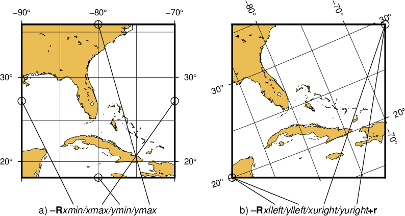
The plot region can be specified in two different ways. (a) Extreme values for each dimension, or (b) coordinates of lower left and upper right corners.

For rectilinear projections the first two forms give identical results. Depending on the selected map projection (or the kind of expected input data), the boundary coordinates may take on several different formats:

Geographic coordinates:

These are longitudes and latitudes and may be given in decimal degrees (e.g., -123.45417) or in the [±]ddd[:mm[:ss[.xxx]]][W|E|S|N] format (e.g., 123:27:15W). Note that -Rg and -Rd are shorthands for “global domain” -R0/360/-90/90 and -R-180/180/-90/90, respectively.

When used in conjunction with the Cartesian Linear Transformation (-Jx or -JX) —which can be used to map floating point data, geographical coordinates, as well as time coordinates— it is prudent to indicate that you are using geographical coordinates in one of the following ways:

Use -Rg or -Rd to indicate the global domain.
Use -Rgxmin/xmax/ymin/ymax to indicate a limited geographic domain.
Add W, E, S, or N to the coordinate limits or add the generic D or G. Example: -R0/360G/-90/90N.

Alternatively, you may indicate geographical coordinates by supplying -fg; see Section Data type selection: The -f option.

Projected coordinates:

These are Cartesian projected coordinates compatible with the chosen projection and are given in a length unit set via the +u modifier, (e.g., -200/200/-300/300+uk for a 400 by 600 km rectangular area centered on the projection center (0, 0). These coordinates are internally converted to the corresponding geographic (longitude, latitude) coordinates for the lower left and upper right corners. This form is convenient when you want to specify a region directly in the projected units (e.g., UTM meters). For allowable units, see Table distunits.

Calendar time coordinates:

These are absolute time coordinates referring to a Gregorian or ISO calendar. The general format is [date]T[clock], where date must be in the yyyy[-mm[-dd]] (year, month, day-of-month) or yyyy[-jjj] (year and day-of-year) for Gregorian calendars and yyyy[-Www[-d]] (year, week, and day-of-week) for the ISO calendar. Note: this format requirement only applies to command-line arguments and not time coordinates given via data files. If no date is given we assume the current day. The T flag is required if a clock is given.

The optional clock string is a 24-hour clock in hh[:mm[:ss[.xxx]]] format. If no clock is given it implies 00:00:00, i.e., the start of the specified day. Note that not all of the specified entities need be present in the data. All calendar date-clock strings are internally represented as double precision seconds since proleptic Gregorian date Monday January 1 00:00:00 0001. Proleptic means we assume that the modern calendar can be extrapolated forward and backward; a year zero is used, and Gregory’s reforms [11] are extrapolated backward. Note that this is not historical.

Relative time coordinates:

These are coordinates which count seconds, hours, days or years relative to a given epoch. A combination of the parameters TIME_EPOCH and TIME_UNIT define the epoch and time unit. The parameter TIME_SYSTEM provides a few shorthands for common combinations of epoch and unit, like j2000 for days since noon of 1 Jan 2000. The default relative time coordinate is that of UNIX computers: seconds since 1 Jan 1970. Denote relative time coordinates by appending the optional lower case t after the value. When it is otherwise apparent that the coordinate is relative time (for example by using the -f switch), the t can be omitted.

Radians:

For angular regions (and increments) specified in radians you may use a set of forms indicating multiples or fractions of \(\pi\). Valid forms are [±][s]pi[f], where s and f are any integer or floating point numbers, e.g., -2pi/2pi3 goes from -360 to 120 degrees (but in radians). When GMT parses one of these forms we alert the labeling machinery to look for certain combinations of pi, limited to npi, 1.5pi, and fractions 3/4, 2/3, 1/2, 1/3, and 1/4 pi. When an annotated value is within roundoff-error of these combinations we typeset the label using the Greek letter for pi and required multiples or fractions.

Other coordinates:

These are simply any coordinates that are not related to geographic or calendar time or relative time and are expected to be simple floating point values such as [±]xxx.xxx[E|e|D|d[±]xx], i.e., regular or exponential notations, with the enhancement to understand FORTRAN double precision output which may use D instead of E for exponents. These values are simply converted as they are to internal representation. [12]

4.2. Coordinate transformations and map projections: The -J option¶

This option selects the coordinate transformation or map projection. The general format is

-J\(\delta\)[parameters/]scale. Here, \(\delta\) is a lower-case letter of the alphabet that selects a particular map projection, the parameters is zero or more slash-delimited projection parameter, and scale is map scale given in distance units per degree or as 1:xxxxx.
-J\(\Delta\)[parameters/]width. Here, \(\Delta\) is an upper-case letter of the alphabet that selects a particular map projection, the parameters is zero or more slash-delimited projection parameter, and width is map width (map height is automatically computed from the implied map scale and region).

Since GMT version 4.3.0, there is an alternative way to specify the projections: use the same abbreviation as in the mapping package Proj4. The options thus either look like:

-Jabbrev/[parameters/]scale. Here, abbrev is a lower-case abbreviation that selects a particular map projection, the parameters is zero or more slash-delimited projection parameter, and scale is map scale given in distance units per degree or as 1:xxxxx.
-JAbbrev/[parameters/]width. Here, Abbrev is an capitalized abbreviation that selects a particular map projection, the parameters is zero or more slash-delimited projection parameter, and width is map width (map height is automatically computed from the implied map scale and region).

The projections available in GMT are presented in Figure The over-30 map projections and coordinate transformations available in GMT. For details on all GMT projections and the required parameters, see the basemap man page. We will also show examples of every projection in the next Chapters, and a quick summary of projection syntax is listed in Projection Specifications.

The over-30 map projections and coordinate transformations available in GMT

4.3. Map frame and axes annotations: The -B option¶

This is potentially the most complicated option in GMT, but most examples of its usage are actually quite simple. We distinguish between to sets of information: Frame settings and Axes parameters. These are set separately by their own -B invocations; hence multiple -B specifications may be specified. The frame settings covers things such as which axes should be plotted, canvas fill, plot title, and what type of gridlines be drawn, whereas the Axes settings deal with annotation, tick, and gridline intervals, axes labels, and annotation units.

The Frame settings are specified by

-B[axes][+b][+gfill][+n][+olon/lat][+ttitle]

Here, the optional axes dictates which of the axes should be drawn and possibly annotated. By default, all 4 map boundaries (or plot axes) are plotted (denoted W, E, S, N). To change this selection, append the codes for those you want (e.g., WSn). In this example, the lower case n denotes to draw the axis and (major and minor) tick marks on the “northern” (top) edge of the plot. The upper case WS will annotate the “western” and “southern” axes with numerals and plot the any axis labels in addition to draw axis/tick-marks. For 3-D plots you can also specify Z or z. By default a single vertical axes will then be plotted at the most suitable map corner. You can override this by appending any combination of corner ids 1234, where 1 represents the lower left corner and the order goes counter-clockwise. Append +b to draw the outline of the 3-D box defined by -R; this modifier is also needed to display gridlines in the x–z, y–z planes. You may paint the map canvas by appending the +gfill modifier [Default is no fill]. If gridlines are specified via the Axes parameters (discussed below) then by default these are referenced to the North pole. If, however, you wish to produce oblique gridlines about another pole you can append +olon/lat to change this behavior (the modifier is ignored if no gridlines are requested). Append +n to have no frame and annotations at all [Default is controlled by the codes]. Finally, you may optionally add +ttitle to place a title that will appear centered above the plot frame.

The Axes settings are specified by

-B[p|s][x|y|z]intervals[+aangle|n|p][+llabel][+pprefix][+uunit]

but you may also split this into two separate invocations for clarity, i.e.,

-B[p|s][x|y|z][+aangle|n|p][+l|Llabel][+pprefix][+s|Sseclabel][+uunit]
-B[p|s][x|y|z]intervals

The first optional flag following -B selects p (rimary) [Default] or s (econdary) axes information (mostly used for time axes annotations). The [x|y|z] flags specify which axes you are providing information for. If none are given then we default to xy. If you wish to give different annotation intervals or labels for the various axes then you must repeat the B option for each axis (If a 3-D basemap is selected with -p and -Jz, use -Bz to give settings for the vertical axis.). To add a label to an axis, just append +llabel (Cartesian projections only). Use +L to force a horizontal label for y-axes (useful for very short labels). For Cartesian axes you may specify an alternate via +s which is used for right or upper axis axis label (with any +l label used for left and bottom axes). If the axis annotation should have a leading text prefix (e.g., dollar sign for those plots of your net worth) you can append +pprefix. For geographic maps the addition of degree symbols, etc. is automatic (and controlled by the GMT default setting FORMAT_GEO_MAP). However, for other plots you can add specific units by adding +uunit. If any of these text strings contain spaces or special characters you will need to enclose them in quotes. Cartesian x-axes also allow for the optional +aangle, which will plot slanted annotations; angle is measured with respect to the horizontal and must be in the -90 <= angle <= 90 range only. Also, +an is a shorthand for normal (i.e., +a90) and +ap for parallel (i.e., +a0) annotations [Default]. For the y-axis, arbitrary angles are not allowed but +an and +ap specify annotations normal [Default] and parallel to the axis, respectively. Note that these defaults can be changed via MAP_ANNOT_ORTHO.

The intervals specification is a concatenated string made up of substrings of the form

[t]stride[phase][u].

The t flag sets the axis item of interest; the available items are listed in Table inttype. Normally, equidistant annotations occur at multiples of stride; you can phase-shift this by appending phase, which can be a positive or negative number.

Flag	Description
a	Annotation and major tick spacing
f	Minor tick spacing
g	Grid line spacing

Note that the appearance of certain time annotations (month-, week-, and day-names) may be affected by the GMT_LANGUAGE, FORMAT_TIME_PRIMARY_MAP, and FORMAT_TIME_SECONDARY_MAP settings.

For automated plots the region may not always be the same and thus it can be difficult to determine the appropriate stride in advance. Here GMT provides the opportunity to auto-select the spacing between the major and minor ticks and the grid lines, by not specifying the stride value. For example, -Bafg will select all three spacings automatically for both axes. In case of longitude–latitude plots, this will keep the spacing the same on both axes. You can also use -Bafg/afg to auto-select them separately. Also note that given the myriad ways of specifying time-axis annotations, the automatic selections may have to be overridden with manual settings to active exactly what you need.

In the case of automatic spacing, when the stride argument is omitted after g, the grid line spacing is chosen the same as the minor tick spacing; unless g is used in consort with a, then the grid lines are spaced the same as the annotations.

The unit flag u can take on one of 18 codes; these are listed in Table units. Almost all of these units are time-axis specific. However, the m and s units will be interpreted as arc minutes and arc seconds, respectively, when a map projection is in effect.

Flag	Unit	Description
Y	year	Plot using all 4 digits
y	year	Plot using last 2 digits
O	month	Format annotation using FORMAT_DATE_MAP
o	month	Plot as 2-digit integer (1–12)
U	ISO week	Format annotation using FORMAT_DATE_MAP
u	ISO week	Plot as 2-digit integer (1–53)
r	Gregorian week	7-day stride from start of week (see TIME_WEEK_START)
K	ISO weekday	Plot name of weekday in selected language
k	weekday	Plot number of day in the week (1–7) (see TIME_WEEK_START)
D	date	Format annotation using FORMAT_DATE_MAP
d	day	Plot day of month (1–31) or day of year (1–366)
		(see FORMAT_DATE_MAP
R	day	Same as d; annotations aligned with week (see TIME_WEEK_START)
H	hour	Format annotation using FORMAT_CLOCK_MAP
h	hour	Plot as 2-digit integer (0–24)
M	minute	Format annotation using FORMAT_CLOCK_MAP
m	minute	Plot as 2-digit integer (0–60)
S	seconds	Format annotation using FORMAT_CLOCK_MAP
s	seconds	Plot as 2-digit integer (0–60)

As mentioned, there may be two levels of annotations. Here, “primary” refers to the annotation that is closest to the axis (this is the primary annotation), while “secondary” refers to the secondary annotation that is plotted further from the axis. The examples below will clarify what is meant. Note that the terms “primary” and “secondary” do not reflect any hierarchical order of units: The “primary” annotation interval is usually smaller (e.g., days) while the “secondary” annotation interval typically is larger (e.g., months).

4.3.1. Geographic basemaps¶

Geographic basemaps may differ from regular plot axis in that some projections support a “fancy” form of axis and is selected by the MAP_FRAME_TYPE setting. The annotations will be formatted according to the FORMAT_GEO_MAP template and MAP_DEGREE_SYMBOL setting. A simple example of part of a basemap is shown in Figure Geographic map border.

Geographic map border using separate selections for annotation, frame, and grid intervals. Formatting of the annotation is controlled by the parameter FORMAT_GEO_MAP in your gmt.conf.

The machinery for primary and secondary annotations introduced for time-series axes can also be utilized for geographic basemaps. This may be used to separate degree annotations from minutes- and seconds-annotations. For a more complicated basemap example using several sets of intervals, including different intervals and pen attributes for grid lines and grid crosses, see Figure Complex basemap.

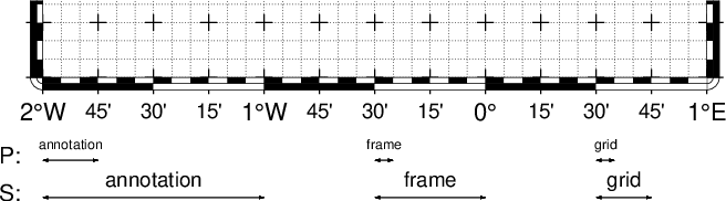
Geographic map border with both primary (P) and secondary (S) components.

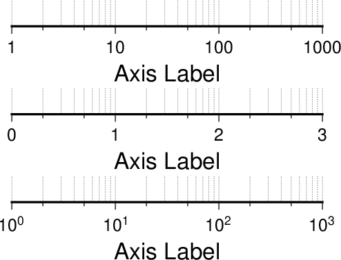
4.3.2. Cartesian linear axes¶

For non-geographic axes, the MAP_FRAME_TYPE setting is implicitly set to plain. Other than that, cartesian linear axes are very similar to geographic axes. The annotation format may be controlled with the FORMAT_FLOAT_OUT parameter. By default, it is set to “%g”, which is a C language format statement for floating point numbers [13], and with this setting the various axis routines will automatically determine how many decimal points should be used by inspecting the stride settings. If FORMAT_FLOAT_OUT is set to another format it will be used directly (.e.g, “%.2f” for a fixed, two decimals format). Note that for these axes you may use the unit setting to add a unit string to each annotation (see Figure Axis label).

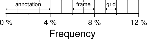
Linear Cartesian projection axis. Long tick-marks accompany annotations, shorter ticks indicate frame interval. The axis label is optional. For this example we used -R0/12/0/0.95 -JX3i/0.3i -Ba4f2g1+lFrequency+u" %" -BS

There are occasions when the length of the annotations are such that placing them horizontally (which is the default) may lead to overprinting or too few annotations. One solution is to request slanted annotations for the x-axis (e.g., Figure Axis label) via the +aangle modifier.

Linear Cartesian projection axis with slanted annotations. For this example we used -R2000/2020/35/45 -JX12c -Bxa2f+a-30 -BS. For the y-axis only the modifier +ap for parallel is allowed.

4.3.3. Cartesian log₁₀ axes¶

Due to the logarithmic nature of annotation spacings, the stride parameter takes on specific meanings. The following concerns are specific to log axes (see Figure Logarithmic projection axis):

stride must be 1, 2, 3, or a negative integer -n. Annotations/ticks will then occur at 1, 1-2-5, or 1,2,3,4,…,9, respectively, for each magnitude range. For -n the annotations will take place every n’th magnitude.
Append l to stride. Then, log₁₀ of the annotation is plotted at every integer log₁₀ value (e.g., x = 100 will be annotated as “2”) [Default annotates x as is].
Append p to stride. Then, annotations appear as 10 raised to log₁₀ of the value (e.g., 10^-5).

Logarithmic projection axis using separate values for annotation, frame, and grid intervals. (top) Here, we have chosen to annotate the actual values. Interval = 1 means every whole power of 10, 2 means 1, 2, 5 times powers of 10, and 3 means every 0.1 times powers of 10. We used -R1/1000/0/1 -JX3il/0.25i -Ba1f2g3. (middle) Here, we have chosen to annotate \(\log_{10}\) of the actual values, with -Ba1f2g3l. (bottom) We annotate every power of 10 using \(\log_{10}\) of the actual values as exponents, with -Ba1f2g3p.

4.3.4. Cartesian exponential axes¶

Normally, stride will be used to create equidistant (in the user’s unit) annotations or ticks, but because of the exponential nature of the axis, such annotations may converge on each other at one end of the axis. To avoid this problem, you can append p to stride, and the annotation interval is expected to be in transformed units, yet the annotation itself will be plotted as un-transformed units (see Figure Power projection axis). E.g., if stride = 1 and power = 0.5 (i.e., sqrt), then equidistant annotations labeled 1, 4, 9, … will appear.

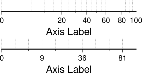
Exponential or power projection axis. (top) Using an exponent of 0.5 yields a \(sqrt(x)\) axis. Here, intervals refer to actual data values, in -R0/100/0/0.9 -JX3ip0.5/0.25i -Ba20f10g5. (bottom) Here, intervals refer to projected values, although the annotation uses the corresponding unprojected values, as in -Ba3f2g1p.

4.3.5. Cartesian time axes¶

What sets time axis apart from the other kinds of plot axes is the numerous ways in which we may want to tick and annotate the axis. Not only do we have both primary and secondary annotation items but we also have interval annotations versus tick-mark annotations, numerous time units, and several ways in which to modify the plot. We will demonstrate this flexibility with a series of examples. While all our examples will only show a single x-axis (south, selected via -BS), time-axis annotations are supported for all axes.

Our first example shows a time period of almost two months in Spring 2000. We want to annotate the month intervals as well as the date at the start of each week:

gmt begin GMT_-B_time1
	gmt set FORMAT_DATE_MAP=-o FONT_ANNOT_PRIMARY +9p
	gmt basemap -R2000-4-1T/2000-5-25T/0/1 -JX5i/0.2i -Bpa7Rf1d -Bsa1O -BS
gmt end show

These commands result in Figure Cartesian time axis. Note the leading hyphen in the FORMAT_DATE_MAP removes leading zeros from calendar items (e.g., 02 becomes 2).

Cartesian time axis, example 1

The next example shows two different ways to annotate an axis portraying 2 days in July 1969:

gmt begin GMT_-B_time2
  gmt set FORMAT_DATE_MAP "o dd" FORMAT_CLOCK_MAP hh:mm FONT_ANNOT_PRIMARY +9p
  gmt basemap -R1969-7-21T/1969-7-23T/0/1 -JX5i/0.2i -Bpa6Hf1h -Bsa1K -BS
  gmt basemap -Bpa6Hf1h -Bsa1D -BS -Y0.65i
gmt end show

The lower example (Figure Cartesian time axis, example 2) chooses to annotate the weekdays (by specifying a1K) while the upper example choses dates (by specifying a1D). Note how the clock format only selects hours and minutes (no seconds) and the date format selects a month name, followed by one space and a two-digit day-of-month number.

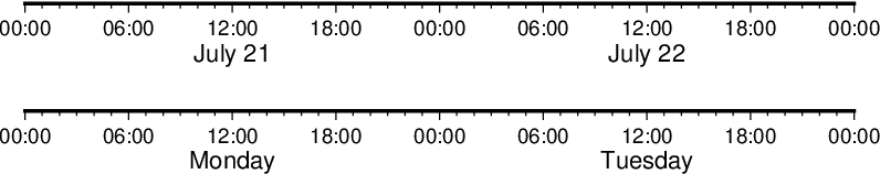
Cartesian time axis, example 2

The third example (Figure Cartesian time axis, example 3) presents two years, annotating both the years and every 3rd month.

gmt begin GMT_-B_time3
	gmt set FORMAT_DATE_MAP o FORMAT_TIME_PRIMARY_MAP Character FONT_ANNOT_PRIMARY +9p
	gmt basemap -R1997T/1999T/0/1 -JX5i/0.2i -Bpa3Of1o -Bsa1Y -BS
gmt end show

Note that while the year annotation is centered on the 1-year interval, the month annotations must be centered on the corresponding month and not the 3-month interval. The FORMAT_DATE_MAP selects month name only and FORMAT_TIME_PRIMARY_MAP selects the 1-character, upper case abbreviation of month names using the current language (selected by GMT_LANGUAGE).

Cartesian time axis, example 3

The fourth example (Figure Cartesian time axis, example 4) only shows a few hours of a day, using relative time by specifying t in the -R option while the TIME_UNIT is d (for days). We select both primary and secondary annotations, ask for a 12-hour clock, and let time go from right to left:

gmt begin GMT_-B_time4
	gmt set FORMAT_CLOCK_MAP=-hham FONT_ANNOT_PRIMARY +9p TIME_UNIT d
	gmt basemap -R0.2t/0.35t/0/1 -JX-5i/0.2i -Bpa15mf5m -Bsa1H -BS
gmt end show

Cartesian time axis, example 4

The fifth example shows a few weeks of time (Figure Cartesian time axis, example 5). The lower axis shows ISO weeks with week numbers and abbreviated names of the weekdays. The upper uses Gregorian weeks (which start at the day chosen by TIME_WEEK_START); they do not have numbers.

gmt begin GMT_-B_time5
	gmt set FORMAT_DATE_MAP u FORMAT_TIME_PRIMARY_MAP Character FORMAT_TIME_SECONDARY_MAP full FONT_ANNOT_PRIMARY +9p
	gmt basemap -R1969-7-21T/1969-8-9T/0/1 -JX5i/0.2i -Bpa1K -Bsa1U -BS
	gmt set FORMAT_DATE_MAP o TIME_WEEK_START Sunday FORMAT_TIME_SECONDARY_MAP Character
	gmt basemap -Bpa3Kf1k -Bsa1r -BS -Y0.65i
gmt end show 

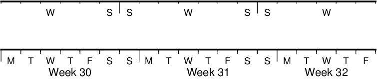
Cartesian time axis, example 5

Our sixth example (Figure Cartesian time axis, example 6) shows the first five months of 1996, and we have annotated each month with an abbreviated, upper case name and 2-digit year. Only the primary axes information is specified.

gmt begin GMT_-B_time6
	gmt set FORMAT_DATE_MAP "o yy" FORMAT_TIME_PRIMARY_MAP Abbreviated
	gmt basemap -R1996T/1996-6T/0/1 -JX5i/0.2i -Ba1Of1d -BS
gmt end show

Cartesian time axis, example 6

Our seventh and final example (Figure Cartesian time axis, example 7) illustrates annotation of year-days. Unless we specify the formatting with a leading hyphen in FORMAT_DATE_MAP we get 3-digit integer days. Note that in order to have the two years annotated we need to allow for the annotation of small fractional intervals; normally such truncated interval must be at least half of a full interval.

gmt begin GMT_-B_time7
	gmt set FORMAT_DATE_MAP jjj TIME_INTERVAL_FRACTION 0.05 FONT_ANNOT_PRIMARY +9p
	gmt basemap -R2000-12-15T/2001-1-15T/0/1 -JX5i/0.2i -Bpa5Df1d -Bsa1Y -BS
gmt end show

Cartesian time axis, example 7

4.3.6. Custom axes¶

Irregularly spaced annotations or annotations based on look-up tables can be implemented using the custom annotation mechanism. Here, we given the c (custom) type to the -B option followed by a filename that contains the annotations (and tick/grid-lines specifications) for one axis. The file can contain any number of comments (lines starting with #) and any number of records of the format

coord type [label]

The coord is the location of the desired annotation, tick, or grid-line, whereas type is a string composed of letters from a (annotation), i interval annotation, f frame tick, and g gridline. You must use either a or i within one file; no mixing is allowed. The coordinates should be arranged in increasing order. If label is given it replaces the normal annotation based on the coord value. Our last example (Figure Custom and irregular annotations) shows such a custom basemap with an interval annotations on the x-axis and irregular annotations on the y-axis.

cat << EOF >| xannots.txt
416.0	ig	Devonian
443.7	ig	Silurian
488.3	ig	Ordovician
542	ig	Cambrian
EOF
cat << EOF >| yannots.txt
0	a
1	a
2	f
2.71828	ag	e
3	f
3.1415926	ag	@~p@~
4	f
5	f
6	f
6.2831852	ag	2@~p@~
EOF

gmt begin GMT_-B_custom
	gmt basemap -R416/542/0/6.2831852 -JX-5i/2.5i -Bpx25f5g25+u" Ma" -Bpycyannots.txt -BWS+glightblue
	gmt basemap -R416/542/0/6.2831852 -JX-5i/2.5i -Bsxcxannots.txt -Bsy0 -BWS \
		--MAP_ANNOT_OFFSET_SECONDARY=10p --MAP_GRID_PEN_SECONDARY=2p
gmt end show

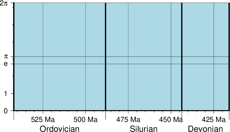
Custom and irregular annotations, tick-marks, and gridlines.

4.4. Timestamps on plots: The -U option¶

The -U option draws the GMT UNIX System time stamp on the plot. By appending +jjust and/or +odx/dy, the user may specify the justification of the stamp and where the stamp should fall on the page relative to lower left corner of the plot. For example, +jBL+o0/0 will align the lower left corner of the time stamp with the bottom left corner of the plot [BL]. Optionally, append an arbitrary text string (surrounded by double quotes), or give +c, which will plot the current command string (Figure Time stamp).

The -U option makes it easy to date a plot.

4.5. Verbose feedback: The -V option¶

The -V option selects verbose mode, which will send progress reports to standard error. Even more verbose levels are -Vl (long verbose) and -Vd (debug). Normal verbosity level produces only error and warning messages. This is the default or can be selected by using -Vn. If compiled with backward-compatibility support, the default is -Vc, which includes warnings about deprecated usage. Finally, -Vq can be used to run without any warnings or errors. This option can also be set by specifying the default GMT_VERBOSE, as quiet, normal, compat, verbose, long_verbose, or debug, in order of increased verbosity.

4.6. Plot positioning and layout: The -X -Y options¶

The -X and -Y options shift origin of plot by (xoff,yoff) inches (Default is (MAP_ORIGIN_X, MAP_ORIGIN_Y) for new plots [15] and (0,0) for overlays. By default, all translations are relative to the previous origin (see Figure Plot positioning). Supply offset as c to center the plot in that direction relative to the page margin. Absolute translations (i.e., relative to a fixed point (0,0) at the lower left corner of the paper) can be achieve by prepending “a” to the offsets. Subsequent overlays will be co-registered with the previous plot unless the origin is shifted using these options. The offsets are measured in the current coordinates system.

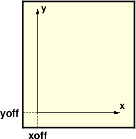
Plot origin can be translated freely with -X -Y.

4.7. OGR/GMT GIS i/o: The -a option¶

GMT relies on external tools to translate geospatial files such as shapefiles into a format we can read. The tool ogr2ogr in the GDAL package can do such translations and preserve the aspatial metadata via a new OGR/GMT format specification (See Chapter The GMT Vector Data Format for OGR Compatibility). For this to be useful we need a mechanism to associate certain metadata values with required input and output columns expected by GMT programs. The -a option allows you to supply one or more comma-separated associations col=name, where name is the name of an aspatial attribute field in a OGR/GMT file and whose value we wish to as data input for column col. The given aspatial field thus replaces any other value already set. Note that col = 0 is the first data columns. Note that if no aspatial attributes are needed then the -a option is not needed – GMT will still process and read such data files.

4.7.1. OGR/GMT input with -a option¶

If you need to populate GMT data columns with (constant) values specified by aspatial attributes, use -a and append any number of comma-separated col=name associations. E.g., 2=depth will read the spatial x,y columns from the file and add a third (z) column based on the value of the aspatial field called depth. You can also associate aspatial fields with other settings such as labels, fill colors, pens, and values used to look-up colors. Do so by letting the col value be one of D, G, L, T, W, or Z. This works analogously to how standard multi-segment files can pass such options via its segment headers (See Chapter GMT File Formats).

4.7.2. OGR/GMT output with -a option¶

You can also make GMT table-writing tools output the OGR/GMT format directly. Again, specify if certain GMT data columns with constant values should be stored as aspatial metadata using the col=name[:type], where you can optionally specify what data type it should be (double, integer, string, logical, byte, or datetime) [double is default]. As for input, you can also use the special col entries of D, G, L, T, W, or Z to have values stored as options in segment headers be used as the source for the name aspatial field. Finally, for output you must append +ggeometry, where geometry can be any of [M]POINT|LINE|POLY; the M represent the multi-versions of these three geometries. Use upper-case +G to signal that you want to split any line or polygon features that straddle the Dateline.

4.8. Binary table i/o: The -b option¶

All GMT programs that accept table data as primary input may read ASCII, native binary, shapefiles, or netCDF tables (Any secondary input files provided via command line options are always expected to be in ASCII format). Native binary files may have a header section and the -hn option (see Section Header data records: The -h option) can be used to skip the first n bytes. The data record can be in any format, you may mix different data types and even byte-swap individual columns or the entire record. When using native binary data the user must be aware of the fact that GMT has no way of determining the actual number of columns in the file. You must therefore pass that information to GMT via the binary -bi nt option, where n is the number of data columns of given type t, where t must be one of c (signed 1-byte character, int8_t), u (unsigned 1-byte character, uint8_t), h (signed 2-byte int, int16_t), H (unsigned 2-byte int, uint16_t), i (signed 4-byte int, int32_t), I (unsigned 4-byte int, uint32_t), l (signed 8-byte int, int64_t), L (unsigned 8-byte int, uint64_t), f (4-byte single-precision float), and d (8-byte double-precision float). In addition, use x to skip n bytes anywhere in the record. For a mixed-type data record you can concatenate several [n]t combinations, separated by commas. You may append w to any of the items to force byte-swapping. Alternatively, append +L|B to indicate that the entire data file should be read or written as little- or big-endian, respectively. Here, n is the number of each item in your binary file. Note that n may be larger than m, the number of columns that the GMT program requires to do its task. If n is not given then it defaults to m and all columns are assumed to be of the single specified type t [d (double), if not set]. If n < m an error is generated. Multiple segment files are allowed and the segment headers are assumed to be records where all the fields equal NaN.

For native binary output, use the -bo option; see -bi for further details.

Because of its meta data, reading netCDF tables (i.e., netCDF files containing 1-dimensional arrays) is quite a bit less complex than reading native binary files. When feeding netCDF tables to programs like plot, the program will automatically recognize the format and read whatever amount of columns are needed for that program. To steer which columns are to be read, the user can append the suffix ?var1/var2/… to the netCDF file name, where var1, var2, etc. are the names of the variables to be processed. No -bi option is needed in this case.

Currently, netCDF tables can only be input, not output. For more information, see Chapter GMT File Formats.

4.9. Missing data conversion: The -d option¶

Within GMT, any missing values are represented by the IEEE NaN value. However, there are occasionally the need to handle user data where missing data are represented by some unlikely data value such as -99999. Since GMT cannot guess that in your data set -99999 is a special value, you can use the -d option to have such values replaced with NaNs. Similarly, should your GMT output need to conform to such a requirement you can replace all NaNs with the chosen nodata value. If only input or output should be affected, use -di or -do, respectably.

4.10. Data record pattern matching: The -e option¶

Modules that read ASCII tables will normally process all the data records that are read. The -e option offers a built-in pattern scanner that will only pass records that match the given patterns or regular expressions. The test can also be inverted to only pass data records that do not match the pattern. The test is not applied to header or segment headers.

4.11. Data type selection: The -f option¶

When map projections are not required we must explicitly state what kind of data each input or output column contains. This is accomplished with the -f option. Following an optional i (for input only) or o (for output only), we append a text string with information about each column (or range of columns) separated by commas. Each string starts with the column number (0 is first column) followed by either x (longitude), y (latitude), T (absolute calendar time) or t (relative time). If several consecutive columns have the same format you may specify a range of columns rather than a single column, i.e., 0–4 for the first 5 columns. For example, if our input file has geographic coordinates (latitude, longitude) with absolute calendar coordinates in the columns 3 and 4, we would specify fi0y,1x,3–4T. All other columns are assumed to have the default, floating point format and need not be set individually. The shorthand -f[i|o]g means -f[i|o]0x,1y (i.e., geographic coordinates). A special use of -f is to select -fp[unit], which requires -J and lets you use projected map coordinates (e.g., UTM meters) as data input. Such coordinates are automatically inverted to longitude, latitude during the data import. Optionally, append a length unit (see Table distunits) [meter]. For more information, see Sections Input data formats and Output data formats.

4.12. Data gap detection: The -g option¶

GMT has several mechanisms that can determine line segmentation. Typically, data segments are separated by multiple segment header records (see Chapter GMT File Formats). However, if key data columns contain a NaN we may also use that information to break lines into multiple segments. This behavior is modified by the parameter IO_NAN_RECORDS which by default is set to skip, meaning such records are considered bad and simply skipped. If you wish such records to indicate a segment boundary then set this parameter to pass. Finally, you may wish to indicate gaps based on the data values themselves. The -g option is used to detect gaps based on one or more criteria (use -ga if all the criteria must be met; otherwise only one of the specified criteria needs to be met to signify a data gap). Gaps can be based on excessive jumps in the x- or y-coordinates (-gx or -gy), or on the distance between points (-gd). Append the gap distance and optionally a unit for actual distances. For geographic data the optional unit may be arc degree, minute, and second, or meter [Default], feet, kilometer, Miles, or nautical miles. For programs that map data to map coordinates you can optionally specify these criteria to apply to the projected coordinates (by using upper-case -gX, -gY or -gD). In that case, choose from centimeter, inch or point [Default unit is controlled by PROJ_LENGTH_UNIT]. Note: For -gx or -gy with time data the unit is instead controlled by TIME_UNIT. Normally, a gap is computed as the absolute value of the specified distance measure (see above). Append +n to compute the gap as previous minus current column value and +p for current minus previous column value.

4.13. Header data records: The -h option¶

The -h[i|o][n_recs] option lets GMT know that input file(s) have n_recs header records [0]. If there are more than one header record you must specify the number after the -h option, e.g., -h4. Note that blank lines and records that start with the character # are automatically considered header records and skipped. Thus, n_recs refers to general text lines that do not start with # and thus must specifically be skipped in order for the programs to function properly. The default number of such header records if -h is used is one of the many parameters in the gmt.conf file (IO_N_HEADER_RECS, by default 0), but can be overridden by -hn_header_recs. Normally, programs that both read and write tables will output the header records that are found on input. Use -hi to suppress the writing of header records. You can use the -h options modifiers to to tell programs to output extra header records for titles, remarks or column names identifying each data column.

When -b is used to indicate binary data the -h takes on a slightly different meaning. Now, the n_recs argument is taken to mean how many bytes should be skipped (on input) or padded with the space character (on output).

4.14. Input columns selection: The -i option¶

The -icolumns option allows you to specify which input file physical data columns to use and in what order. By default, GMT will read all the data columns in the file, starting with the first column (0). Using -i modifies that process and reads in a logical record based on columns from the physical record. For instance, to use the 4th, 7th, and 3rd data column as the required x,y,z to blockmean you would specify -i3,6,2 (since 0 is the first column). The chosen data columns will be used as is. Optionally, you can specify that input columns should be transformed according to a linear or logarithmic conversion. Do so by appending [+l][+sscale][+ooffset] to each column (or range of columns). All items are optional: The +l implies we should first take \(\log_{10}\) of the data [leave as is]. Next, we may scale the result by the given scale [1]. Finally, we add in the specified offset [0]. If you want the trailing text to remain part of your subset logical record then also select the special column by requesting column t, otherwise we ignore trailing text. If you only want to select one word from the trailing text, then append the word number (0 is the first word). Finally, to use the entire numerical record and ignore trailing text, use -in.

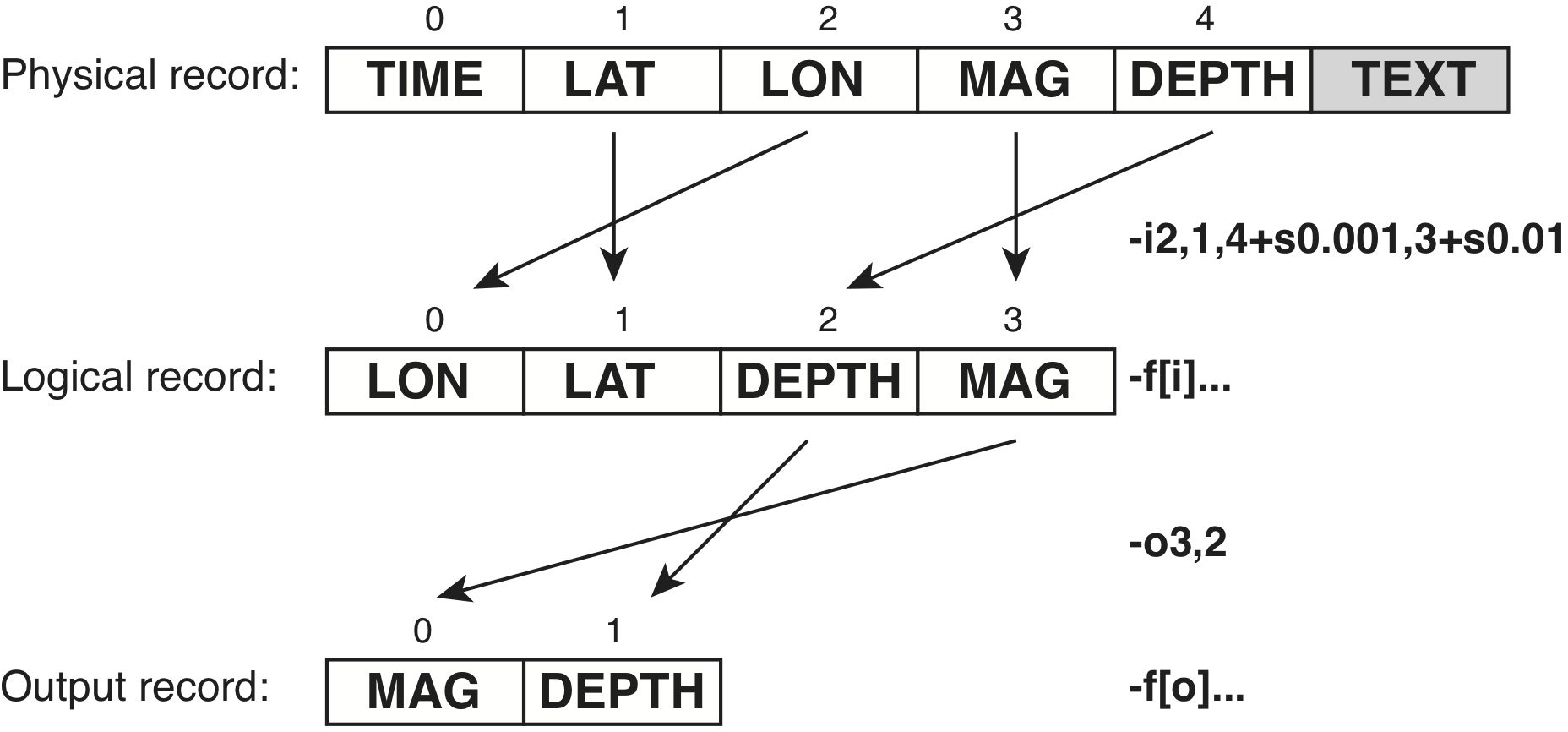
The physical, logical (input) and output record in GMT. Here, we are reading a file with 5 numerical columns plus some free-form text at the end. Our module (here plot) will be used to plot circles at the given locations but we want to assign color based on the depth column (which we need to convert from meters to km) and symbol size based on the mag column (but we want to scale the magnitude by 0.01 to get suitable symbol sizes). We use -i to pull in the desired columns in the required order and apply the scaling, resulting in a logical input record with 4 columns. The -f option can be used to specify column types in the logical record if it is not clear from the data themselves (such as when reading a binary file). Finally, if a module needs to write out only a portion of the current logical record then you may use the corresponding -o option to select desired columns, including the trailing text column t. If you only want to output one word from the trailing text, then append the word number (0 is the first word). Note that these column numbers now refer to the logical record, not the physical, since after reading the data there is no physical record, only the logical record in memory.

. _option_-j:

4.15. Spherical distance calculations: The -j option¶

GMT has different ways to compute distances on planetary bodies. By default (-jg) we perform great circle distance calculations, and parameters such as distance increments or radii will be compared against calculated great circle distances. To simplify and speed up calculations you can select Flat Earth mode (-jf) instead, which gives an approximate but faster result. Alternatively, you can select ellipsoidal (-je; i.e., geodesic) mode for the highest precision (and slowest calculation time). All spherical distance calculations depend on the current ellipsoid (PROJ_ELLIPSOID), the definition of the mean radius (PROJ_MEAN_RADIUS), and the specification of latitude type (PROJ_AUX_LATITUDE). Geodesic distance calculations is also controlled by method (PROJ_GEODESIC).

4.16. Setting automatic legend entries: The -l option¶

Map or plot legends are created by legend and normally this module will read a specfile that outlines how the legend should look. You can make very detailed and complicated legends by mixing a variety of items, such as symbol, free text, colorbars, scales, images, and more. Yet, for the vast majority of plots displaying symbols or lines a simple legend will suffice. The -l option is used to automatically build the specfile as we plot the various layers that will make up our illustration. Apart from setting the label string that goes with the current symbol or line, you can select from a series of modifiers that mirror the effect of control codes normally added to the specfile by hand. For instance, a simple plot with two symbols can obtain a legend by using this option and modifiers and is shown in Figure Auto Legend:

gmt begin fruit
  gmt plot -R0/7.2/3/7.2 -Jx2c @Table_5_11.txt -Sc0.35c -Glightgreen -Wfaint -lApples+h"LEGEND"+f16p+d
  gmt plot @Table_5_11.txt -St0.35c -Gorange -B -BWStr -lOranges
  gmt legend -DjTR+w3c+o0.25c -F+p1p+ggray95+s
gmt end show

As the script shows, when no specfile is given to legend then we look for the automatically generated on in the session directory.

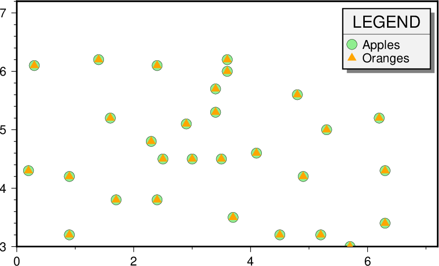
Each of the two plot commands use -l to add a symbol to the auto legend; the first also sets a legend header of given size and draws a horizontal line.

4.17. Grid interpolation parameters: The -n option¶

The -ntype option controls parameters used for 2-D grids resampling. You can select the type of spline used (-nb for B-spline smoothing, -nc for bicubic [Default], -nl for bilinear, or -nn for nearest-node value). For programs that support it, antialiasing is by default on; optionally, append +a to switch off antialiasing. By default, boundary conditions are set according to the grid type and extent. Change boundary conditions by appending +bBC, where BC is either g for geographic boundary conditions or one (or both) of n and p for natural or periodic boundary conditions, respectively. Append x or y to only apply the condition in one dimension. E.g., -nb+nxpy would imply natural boundary conditions in the x direction and periodic conditions in the y direction. Finally, append +tthreshold to control how close to nodes with NaN the interpolation should go. A threshold of 1.0 requires all (4 or 16) nodes involved in the interpolation to be non-NaN. 0.5 will interpolate about half way from a non-NaN value; 0.1 will go about 90% of the way, etc.

4.18. Output columns selection: The -o option¶

The -ocolumns option allows you to specify which columns to write on output and in what order. By default, GMT will write all the data columns produced by the program. Using -o modifies that process. For instance, to write just the 4th and 2nd data column to the output you would use -o3,1 (since 0 is the first column). You can also use a column more than once, e.g., -o3,1,3, to duplicate a column on output. Finally, if your logical record in memory contains trailing text then you can include that by including the special column t to your selections. The text is always written after any numerical columns. If you only want to output one word from the trailing text, then append the word number (0 is the first word). Note that if you wanted to scale or shift the output values you need to do so during reading, using the -i option. To output all numerical columns and ignoring trailing text, use -on.

4.19. Perspective view: The -p option¶

All plotting programs that normally produce a flat, two-dimensional illustration can be told to view this flat illustration from a particular vantage point, resulting in a perspective view. You can select perspective view with the -p option by setting the azimuth and elevation of the viewpoint [Default is 180/90]. When -p is used in consort with -Jz or -JZ, a third value can be appended which indicates at which z-level all 2-D material, like the plot frame, is plotted (in perspective) [Default is at the bottom of the z-axis]. For frames used for animation, you may want to append + to fix the center of your data domain (or specify a particular world coordinate point with +wlon0/lat[z]) which will project to the center of your page size (or you may specify the coordinates of the projected view point with +vx0/y0. When -p is used without any further arguments, the values from the last use of -p in a previous GMT command will be used. Alternatively, you can perform a simple rotation about the z-axis by just giving the rotation angle. Optionally, use +v or +w to select another axis location than the plot origin.

4.20. Grid registration: The -r option¶

All 2-D grids in GMT have their nodes organized in one of two ways, known as gridline- and pixel- registration. The GMT default is gridline registration; programs that allow for the creation of grids can use the -r option (or -rp) to select pixel registration instead. Most observed data tend to be in gridline registration while processed data sometime may be distributed in pixel registration. While you may convert between the two registrations this conversion looses the Nyquist frequency and dampens the other high frequencies. It is best to avoid any registration conversion if you can help it. Planning ahead may be important.

4.20.1. Gridline registration¶

In this registration, the nodes are centered on the grid line intersections and the data points represent the average value in a cell of dimensions (\(x_{inc} \cdot y_{inc}\)) centered on each node (left side of Figure Grid registration). In the case of grid line registration the number of nodes are related to region and grid spacing by

\[\begin{split}\begin{array}{ccl} nx & = & (x_{max} - x_{min}) / x_{inc} + 1 \\ ny & = & (y_{max} - y_{min}) / y_{inc} + 1 \end{array}\end{split}\]

which for the example in left side of Figure Gridline registration yields nx = ny = 4.

4.20.2. Pixel registration¶

Here, the nodes are centered in the grid cells, i.e., the areas between grid lines, and the data points represent the average values within each cell (right side of Figure Grid registration). In the case of pixel registration the number of nodes are related to region and grid spacing by

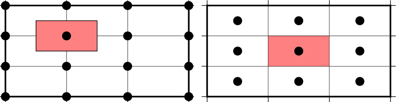
Gridline- and pixel-registration of data nodes. The red shade indicates the areas represented by the value at the node (solid circle).

\[\begin{split}\begin{array}{ccl} nx & = & (x_{max} - x_{min}) / x_{inc} \\ ny & = & (y_{max} - y_{min}) / y_{inc} \end{array}\end{split}\]

Thus, given the same region (-R) and grid spacing, the pixel-registered grids have one less column and one less row than the gridline-registered grids; here we find nx = ny = 3.

4.21. NaN-record treatment: The -s option¶

We can use this option to suppress output for records whose z-value equals NaN (by default we output all records). Alternatively, append +r to reverse the suppression, i.e., only output the records whose z-value equals NaN. Use -s+a to suppress output records where one or more fields (and not necessarily z) equal NaN. Finally, you can supply a comma-separated list of all columns or column ranges to consider (before the optional modifiers) for this NaN test.

4.22. Layer transparency: The -t option¶

While the PostScript language does not support transparency, PDF does, and via PostScript extensions one can manipulate the transparency levels of objects. The -t option allows you to change the transparency level for the current overlay by appending a percentage in the 0-100 range; the default is 0, or opaque. Transparency may also be controlled on a feature by feature basis when setting color or fill (see section Specifying area fill attributes). Finally, the modules plot, plot3d, and text can all change transparency on a record-by-record basis if -t is given without argument and the input file supplies variable transparencies as the last numerical column value.

4.23. Latitude/Longitude or Longitude/Latitude?: The -: option¶

For geographical data, the first column is expected to contain longitudes and the second to contain latitudes. To reverse this expectation you must apply the -: option. Optionally, append i or o to restrict the effect to input or output only. Note that command line arguments that may take geographic coordinates (e.g., -R) always expect longitude before latitude. Also, geographical grids are expected to have the longitude as first (minor) dimension.

[11]

The Gregorian Calendar is a revision of the Julian Calendar which was instituted in a papal bull by Pope Gregory XIII in 1582. The reason for the calendar change was to correct for drift in the dates of significant religious observations (primarily Easter) and to prevent further drift in the dates. The important effects of the change were (a) Drop 10 days from October 1582 to realign the Vernal Equinox with 21 March, (b) change leap year selection so that not all years ending in “00” are leap years, and (c) change the beginning of the year to 1 January from 25 March. Adoption of the new calendar was essentially immediate within Catholic countries. In the Protestant countries, where papal authority was neither recognized not appreciated, adoption came more slowly. England finally adopted the new calendar in 1752, with eleven days removed from September. The additional day came because the old and new calendars disagreed on whether 1700 was a leap year, so the Julian calendar had to be adjusted by one more day.

[12]	While UTM coordinates clearly refer to points on the Earth, in this context they are considered “other”. Thus, when we refer to “geographical” coordinates herein we imply longitude, latitude.

[13]	Please consult the man page for printf or any book on C.

[15]	Ensures that boundary annotations do not fall off the page.