gravprisms
Compute geopotential anomalies over 3-D vertical prisms
Synopsis
gmt gravprisms [ table ] [ -C[+q][+wfile][+zdz] ] [ -Ddensity[+c] ] [ -Edx[/dy] ] [ -Ff|n[lat]|v ] [ -Goutfile ] [ -HH/rho_l/rho_h[+bboost][+ddensify][+ppower] ] [ -Iincrement ] [ -Lbase ] [ -M[h][v] ] [ -Ntrackfile ] [ -Rregion ] [ -Sshapegrid ] [ -Ttop ] [ -V[level] ] [ -Wavedens ] [ -Zlevel|obsgrid ] [ -bobinary ] [ -dnodata[+ccol] ] [ -eregexp ] [ -fflags ] [ -iflags ] [ -oflags ] [ -rreg ] [ -x[[-]n] ] [ --PAR=value ]
Note: No space is allowed between the option flag and the associated arguments.
Description
gravprisms will compute the geopotential field over vertically oriented, rectangular prisms. We either read the multi-segment table from file (or standard input), which may contain up to 7 columns: The first four are x y z_low z_high, i.e., the center x, y coordinates and the vertical range of the prism from z_low to z_high, while the next two columns hold the dimensions dx dy of each prism (see -E if all prisms have the same x- and y-dimensions). Last column may contain individual prism densities (but will be overridden by fixed or variable density contrasts if given via -D). Alternatively, we can use -C to create the prisms needed to approximate the entire feature (-S) or just the volume between two surfaces (one of which may be a constant) that define a layer (set via -L and -T). If a variable density model (-H) is selected then each vertical prism will be broken into constant-density, stacked sub-prisms using a prescribed vertical increment dz, otherwise single tall prisms are created with constant or spatially variable densities (-D). We can compute anomalies on an equidistant grid (by specifying a new grid with -R and -I or provide an observation grid with desired elevations) or at arbitrary output points specified via -N. Choose between free-air anomalies, vertical gravity gradient anomalies, or geoid anomalies. Options are available to control axes units and direction.
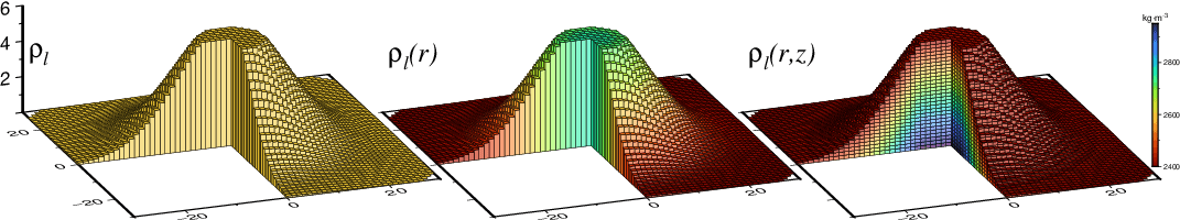
Three density models modeled by prisms for a truncated Gaussian seamount via -C: (left) Constant density (-D), (middle) vertically-averaged density varying radially (-D), and (right) density varies with r and z (-H), requiring a stack of prisms.
Required Arguments
- table
The file describing the prisms with record format x y z_lo z_hi [ dx dy ] [ rho ], where the optional items are controlled by options -E and -D, respectively. Density contrasts can be given in \(\mbox{kg/m}^3\) of \(\mbox{g/cm}^3\). Note: If -C is used then no table will be read.
- -Ix_inc[+e|n][/y_inc[+e|n]]
Set the grid spacing as x_inc [and optionally y_inc].
Geographical (degrees) coordinates: Optionally, append an increment unit. Choose among:
d - Indicate arc degrees
m - Indicate arc minutes
s - Indicate arc seconds
If one of e (meter), f (foot), k (km), M (mile), n (nautical mile) or u (US survey foot), the increment will be converted to the equivalent degrees longitude at the middle latitude of the region (the conversion depends on PROJ_ELLIPSOID). If y_inc is not given or given but set to 0 it will be reset equal to x_inc; otherwise it will be converted to degrees latitude.
All coordinates: The following modifiers are supported:
+e - Slightly adjust the max x (east) or y (north) to fit exactly the given increment if needed [Default is to slightly adjust the increment to fit the given domain].
+n - Define the number of nodes rather than the increment, in which case the increment is recalculated from the number of nodes, the registration (see GMT File Formats), and the domain. Note: If -Rgrdfile is used then the grid spacing and the registration have already been initialized; use -I and -R to override these values.
- -Rxmin/xmax/ymin/ymax[+r][+uunit]
Specify the region of interest. (See full description) (See technical reference).
Optional Arguments
- -C[+q][+wfile][+zdz] ]
Create prisms for the entire feature given by -Sheight, or just for the layer between the two surfaces specified via -Lbase and -Ttop. For layers, either base or top may be a constant rather than a grid. If only height is given then we assume we will approximate the entire feature from base = 0 to height. If -H is used to compute variable density contrasts then we must split each prism into a stack of sub-prisms with individual densities. This is controlled via these modifiers:
+q - Quit execution once that file set with +w has been saved, i.e., no geopotential calculations will take place.
+w - Append file to save the prisms to a table.
+z - Append dz for the heights of these sub-prisms (the first and last sub-prisms in the stack may have their heights adjusted to match the limits of the surfaces). Without -H we only create a single uniform-density prism, but those prisms may have spatially varying densities via a grid given in -D.
- -Ddensity[+c]
Sets a fixed density contrast that overrides any individual prism settings in the prisms file, in \(\mbox{kg/m}^3\) of \(\mbox{g/cm}^3\). Append +c to instead subtract this density from the individual prism densities. Alternatively, give name of an input grid with spatially varying, vertically-averaged prism densities. This requires -C and the grid must be co-registered with the grid provided by -S (or -L and -T). Note: If -H is used then a fixed density may be set via -D provided its modifier +c is set. We will then compute density contrasts in the seamount relative to the fixed density (such as density of seawater for underwater seamounts).
- -Edx[/dy]
If all prisms in table have constant x/y-dimensions then they can be set here. In that case table must only contain the centers of each prism and the z range (and optionally density; see -D). If only dx is given then we set dy = dx. Note: For geographic coordinates the dx dimension is in geographic longitude increment and hence the physical width of the prism will decrease with latitude if dx stays numerically the same.
- -Ff|n[lat]|v
Specify desired gravitational field component. Choose between f (free-air anomaly) [Default], n (geoid; optionally append average latitude for normal gravity reference value [Default is mid-grid (or mid-profile if -N)]) or v (vertical gravity gradient).
- -Goutfile
Specify the name of the output data (for grids, see Grid File Formats). Required when an equidistant grid is implied for output. If -N is used then output is written to standard output unless -G specifies an output table name.
- -HH/rho_l/rho_h[+bboost][+ddensify][+ppower]
Set reference seamount parameters for an ad-hoc variable radial density function with depth. Give the rho_l and rho_h seamount densities in \(\mbox{kg/m}^3\) or \(\mbox{g/cm}^3\) and the fixed reference height H in meters. Modifiers can be used for further changes:
+b - Simulate the higher starting densities in truncated guyots. You can boost the seamount height by this factor [1]. Requires -S to know the full height of the seamount.
+d - Change the water-pressure-driven flank densify gradient over the full reference height [0].
+p - Change variable density profile exponent power [Default is 1, i.e., a linear change].
See grdseamount for more details.
- -Lbase
Give name of the base surface grid for a layer we wish to approximate with prisms, or give a constant z-level [0].
- -M[h][v]
Sets distance units used. Append h to indicate that both horizontal distances are in km [m], and append v to indicate vertical distances are in km [m]. If selected, we will internally convert any affected distance provided by data input or command line options to meters. Note: Any output will retain the original units.
- -Ntrackfile
Specifies individual (x, y[, z]) locations where we wish to compute the predicted value. When this option is used there are no grids involved and the output data records are written to standard output (see -bo for binary output). If -Z is not set then trackfile must have 3 columns and we take the z value as our observation level; otherwise s constant level must be set via -Z. Note: If -G is used to set an output file we will write the output table to that file instead of standard output.
- -Sheight
Give name of grid with the full seamount heights, either for making prisms or as required by -H.
- -Ttop
Give name of the top surface grid for a layer we wish to approximate with prisms, or give a constant z-level.
- -V[level]
Select verbosity level [w]. (See full description) (See technical reference).
- -Wavedens
Give name of an output grid with spatially varying, vertically-averaged prism densities created by -C and -H.
- -Zlevel|obsgrid
Set observation level, either as a constant or variable by giving the name of a grid with observation levels. If the latter is used then this grid determines the output grid region as well [0]. Note: the positive z-direction is up.
- -borecord[+b|l] (more …)
Select native binary format for table output. [Default is 2 output columns].
- -d[i|o][+ccol]nodata (more …)
Replace input columns that equal nodata with NaN and do the reverse on output.
- -e[~]“pattern” | -e[~]/regexp/[i] (more …)
Only accept data records that match the given pattern.
- -fflags
Geographic grids (i.e., dimensions of longitude, latitude) will be converted to km via a “Flat Earth” approximation using the current ellipsoidal parameters.
- -h[i|o][n][+c][+d][+msegheader][+rremark][+ttitle] (more …)
Skip or produce header record(s). Not used with binary data.
- -icols[+l][+ddivisor][+sscale|d|k][+ooffset][,…][,t[word]] (more …)
Select input columns and transformations (0 is first column, t is trailing text, append word to read one word only).
- -ocols[+l][+ddivisor][+sscale|d|k][+ooffset][,…][,t[word]] (more …)
Select output columns and transformations (0 is first column, t is trailing text, append word to write one word only).
- -r[g|p] (more …)
Set node registration [gridline].
- -x[[-]n] (more …)
Limit number of cores used in multi-threaded algorithms. Multi-threaded behavior is enabled by default. That covers the modules that implement the OpenMP API (required at compiling stage) and GThreads (Glib) for the grdfilter module.
- -:[i|o] (more …)
Swap 1st and 2nd column on input and/or output.
- -^ or just -
Print a short message about the syntax of the command, then exit (Note: on Windows just use -).
- -+ or just +
Print an extensive usage (help) message, including the explanation of any module-specific option (but not the GMT common options), then exit.
- -? or no arguments
Print a complete usage (help) message, including the explanation of all options, then exit.
- --PAR=value
Temporarily override a GMT default setting; repeatable. See gmt.conf for parameters.
Units
For map distance unit, append unit d for arc degree, m for arc minute, and s for arc second, or e for meter [Default unless stated otherwise], f for foot, k for km, M for statute mile, n for nautical mile, and u for US survey foot. By default we compute such distances using a spherical approximation with great circles (-jg) using the authalic radius (see PROJ_MEAN_RADIUS). You can use -jf to perform “Flat Earth” calculations (quicker but less accurate) or -je to perform exact geodesic calculations (slower but more accurate; see PROJ_GEODESIC for method used).
Examples
We have prepared a set of 2828 prisms that represent a truncated Gaussian seamount of height 6000 m, radius 30 km, with the base at z = 0 m, available in the remote file @prisms.txt. A quick view of the 3-D model can be had via:
gmt plot3d -R-30/30/-30/30/0/7000 -JX12c -JZ3c -Ggray -So1q+b @prisms.txt -B -Wfaint -p200/20 -pdf smt
To compute the free-air anomalies on a grid over the set of prisms given in @prisms.txt, using 1700 \(\mbox{kg/m}^3\) as a fixed density contrast, with horizontal distances in km and vertical distances in meters, observed at 7000 m, try:
gmt gravprisms -R-40/40/-40/40 -I1 -Mh -G3dgrav.nc @prisms.txt -D1700 -Ff -Z7000
gmt grdimage 3dgrav.nc -B -pdf 3dgrav
To obtain the vertical gravity gradient anomaly along the track given in crossing.txt for the same model, try:
gmt math -T-30/30/0.1 T 0 MUL = crossing.txt
gmt gravprisms -Ncrossing.txt -Mh @prisms.txt -D1700 -Fv -Z7000 > vgg_crossing.txt
gmt plot vgg_crossing.txt -R-30/30/-50/400 -i0,3 -W1p -B -pdf vgg_crossing
Finally, redo the gravity calculation but now use the individual prism densities in the prism file and restrict calculations to the same crossing profile, i.e.:
gmt gravprisms -Ncrossing.txt -Mh @prisms.txt -Ff -Z7000 > faa_crossing.txt
gmt plot faa_crossing.txt -R-30/30/0/350 -i0,3 -W1p -B -pdf faa_crossing
To build prisms using a variable density grid for an interface crossing the zero level and obtain prisms with the negative of the given density contrast if below zero and the positive density contrast if above zero, try:
gmt gravprisms -TFlexure_surf.grd -C+wprisms_var.txt+q -DVariable_drho.grd
Geometry Setup
We operate in a right-handed coordinate system where the positive z-axis is directed upwards. In this scenario, topographic surfaces may be above or below a reference surface (typically the observation level) but the positive direction is always up. Positive geopotential anomalies are thus aligned with the positive source (topographic relief) direction. If your input data are positive down (e.g., depths) then you will need to change the sign. For grids you can use the +s and +o modifiers to scale and offset the grid, while for table data you can use the -i modifier to scale and offset any column required.
Grids Straddling Zero Level
When creating prisms from grids via -C, a special case arises when a single surface (set via -L or -T) straddles zero. This may happen if the surface reflects flexure beneath a load, which has in a negative moat flanked by positive bulges. When such a interface grid is detected we build prisms going from z to zero for negative z and from 0 to z for positive z. As we flip below zero we also change the sign of the given density contrast. You can override this behavior by specifying the opposite layer surface either by a constant or another grid. E.g., if -L specifies the base surface you can eliminate prisms exceeding zero via -T0, and by interchanging the -L and -T arguments you can eliminate prisms below zero. Note: When two surfaces are implied we keep the given density contrast as given.
Note on Precision
The analytical expression for the geoid over a vertical prism (Nagy et al., 2000) is fairly involved and contains 48 terms. Due to various cancellations the end result is more unstable than the simpler expressions for gravity and VGG. Be aware that the result may have less significant digits that you may expect.
References
Grant, F. S. and West, G. F., 1965, Interpretation Theory in Applied Geophysics, 583 pp., McGraw-Hill.
Kim, S.-S., and P. Wessel, 2016, New analytic solutions for modeling vertical gravity gradient anomalies, Geochem. Geophys. Geosyst., 17, https://doi.org/10.1002/2016GC006263.
Nagy D., Papp G., Benedek J., 2000, The gravitational potential and its derivatives for the prism, J. Geod., 74, 552–560, https://doi.org/10.1007/s001900000116.
See Also
gmt.conf, gmt, grdmath, gravfft, gmtgravmag3d, grdgravmag3d, grdseamount, talwani2d, talwani3d