grdseamount

Create synthetic seamounts (Gaussian, parabolic, polynomial, cone or disc; circular or elliptical)

Synopsis

gmt grdseamount [ table ] -Goutgrid -Iincrement -Rregion [ -A[out/in][+sscale] ] [ -C[c|d|g|o|p] ] [ -Dunit ] [ -E ] [ -F[flattening] ] [ -HH/rho_l/rho_h[+ddensify][+bboost][+ppower] ] [ -K[densitymodel] ] [ -L[hn] ] [ -M[list] ] [ -Nnorm ] [ -Qbmode[/fmode][+d] ] [ -S[+a[az1/az2]][+b[beta]][+d[hc]][+h[h1/h2]][+p[power]][+t[t0/t1]][+u[u0]][+v[phi]] ] [ -Tt0[/t1/dt][+l] ] [ -Zlevel ] [ -V[level] ] [ -Wavedensity ] [ -bibinary ] [ -eregexp ] [ -fflags ] [ -iflags ] [ -rreg ] [ --PAR=value ]

Note: No space is allowed between the option flag and the associated arguments.

Description

grdseamount will compute the combined topographic shape of multiple synthetic seamounts given their individual shape parameters. We read from table (or standard input) a list of seamount locations and sizes and can evaluate either Gaussian, parabolic, conical, polynomial or disc shapes, which may be circular or elliptical, and optionally truncated. Various options are available to modify the result, including an option to add in a background depth or set unmodified nodes to NaN (more complicated backgrounds may be added separately via grdmath). The input data must contain lon, lat, radius, height for each seamount. For elliptical features (requires -E), we expect lon, lat, azimuth, semi-major, semi-minor, height instead. If flat seamount tops is specified (via -F) with no value appended, then an extra column with flattening is expected (-F cannot be used for plateaus). For temporal evolution of topography the -T option may be used, in which case the data file must have two additional columns with the start and stop time of seamount construction. In this case, you may choose to write out a cumulative shape or just the increments produced for each time step (see -Q). If land slides are considered (-S), then this initial set of input columns are followed by one or more groups of slide parameters; see -S for the arrangement. Finally, for mixing different seamount shapes in the input table you can use the trailing text to give the shape code by using -C without appending an argument.

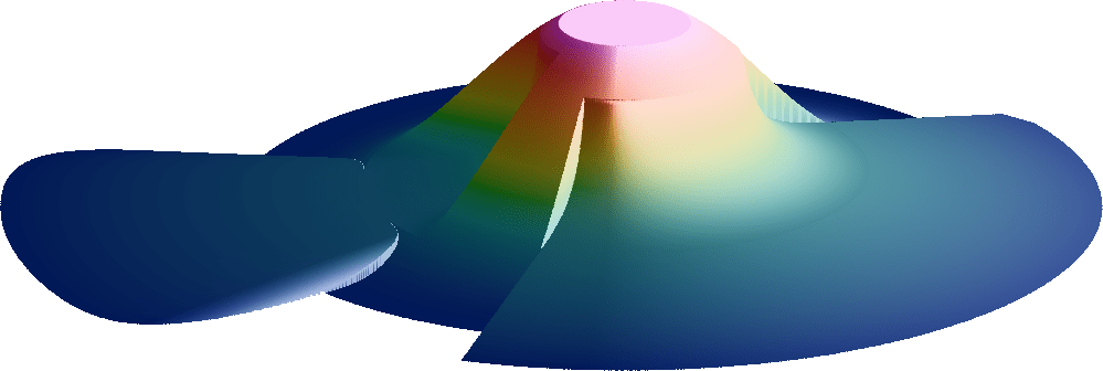
Truncated polynomial seamount with the scars of two mass-wasting events on its flank. Users can assign a time-span to the construction of the seamount and separate time-spans for any desired mass-wasting events.

Required Arguments (if -L is not given)

table

One or more ASCII (or binary, see -bi[ncols][type]) data table file(s) holding a number of data columns. If no tables are given then we read from standard input.

-Goutgrid[=ID][+ddivisor][+ninvalid][+ooffset|a][+sscale|a][:driver[dataType][+coptions]]

Optionally, append =ID for writing a specific file format. The following modifiers are supported:

• +d - Divide data values by given divisor [Default is 1].

• +n - Replace data values matching invalid with a NaN.

• +o - Offset data values by the given offset, or append a for automatic range offset to preserve precision for integer grids [Default is 0].

• +s - Scale data values by the given scale, or append a for automatic scaling to preserve precision for integer grids [Default is 1].

Note: Any offset is added before any scaling. +sa also sets +oa (unless overridden). To write specific formats via GDAL, use =gd and supply driver (and optionally dataType) and/or one or more concatenated GDAL -co options using +c. See the “Writing grids and images” cookbook section for more details.

-Ix_inc[+e|n][/y_inc[+e|n]]

Set the grid spacing as x_inc [and optionally y_inc].

Geographical (degrees) coordinates: Optionally, append an increment unit. Choose among:

• d - Indicate arc degrees

• m - Indicate arc minutes

• s - Indicate arc seconds

If one of e (meter), f (foot), k (km), M (mile), n (nautical mile) or u (US survey foot), the increment will be converted to the equivalent degrees longitude at the middle latitude of the region (the conversion depends on PROJ_ELLIPSOID). If y_inc is not given or given but set to 0 it will be reset equal to x_inc; otherwise it will be converted to degrees latitude.

All coordinates: The following modifiers are supported:

• +e - Slightly adjust the max x (east) or y (north) to fit exactly the given increment if needed [Default is to slightly adjust the increment to fit the given domain].

• +n - Define the number of nodes rather than the increment, in which case the increment is recalculated from the number of nodes, the registration (see GMT File Formats), and the domain. Note: If -Rgrdfile is used then the grid spacing and the registration have already been initialized; use -I and -R to override these values.

-Rxmin/xmax/ymin/ymax[+r][+uunit]

Specify the region of interest. (See full description) (See technical reference).

Optional Arguments

-A[out/in][+sscale]

Build a mask grid only that may be used to manipulate gridded data sets to exclude or to isolate seamount observations; append outside/inside values [1/NaN]. Here, height and flattening are ignored and -L, -N and -Z are disallowed. Optionally, use +s to increase all seamount radii or semi-axes first (e.g., “bleeding the mask outwards”) [1].

-C[c|d|g|o|p]

Select a seamount shape function: choose among c (cone), d (disc), g (Gaussian) o (polynomial) and p (parabola) [Default is Gaussian]. All but the disc can furthermore be truncated via a flattening parameter f set by -F. If -C is not given any argument, then we will read the shape code from the input file’s trailing text. If -C is not given at all, then we default to Gaussian seamounts [g]. Note: The polynomial model has a normalized amplitude v for a normalized radius \(u = r / r_0\) that is given by \(v(u) = (1+u)^3(1-u)^3/(1+u^3)\). It is comparable to the Gaussian model (its volume is just ~2.4% larger), and v goes exactly to zero at the basal radius \(r_0\).

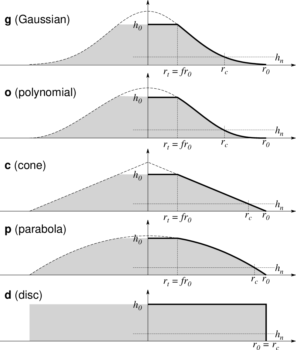
The five types of seamounts selected via option -C. In all cases, \(h_0\) is the maximum height, \(r_0\) is the basal radius, \(h_n\) is the noise floor set via -L [0], and f is the flattening set via -F [0]. The top radius \(r_t = f r_0\) is only nonzero if there is flattening, hence it does not apply to the disc model.

-Dunit

Append the Cartesian unit used for horizontal distances in the input file (see Units). Not allowed for geographic data, which we automatically convert to km using a flat Earth assumption.

-E

Set elliptical data file format. We expect input records to contain (lon, lat, azimuth, semi-major, semi-minor, height) (with the latter in meter) for each seamount [Default is Circular data format, expecting lon, lat, radius, height]. To mix circular and elliptical seamounts you must use -E and provide the circular parameters as elliptical ones via azimuth = 0 and semi-major = semi-minor = radius.

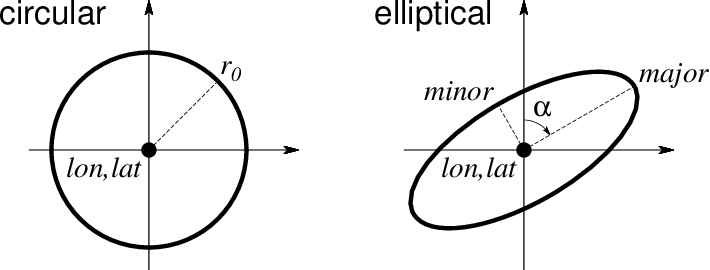
Use -E to select elliptical rather than circular shapes in map view. Both shapes require (lon, lat). Circular shapes only require the radius \(r_0\), while elliptical ones require the azimuth \(\alpha\) of the major axis as well as the major and minor semi-axes .

-F[flattening]

Seamounts will be truncated to guyots. Append flattening from 0 (no flattening) up to, but not including, 1. If no argument is given then we expect to find the flattening in the last input column [no truncation]. Ignored if used with -Cd.

-HH/rho_l/rho_h[+bboost][+ddensify][+ppower]

Set reference seamount parameters for an ad-hoc variable radial density function with depth. Give the low and high seamount densities in \(\mbox{kg/m}^3\) or \(\mbox{g/cm}^3\) and the fixed reference height H in meters. Use modifiers +d and +p to change the water-pressure-driven flank density increase over the full reference height [0] and set the variable density profile exponent power [1, i.e., a linear change]. Below, h(r) is the final height of any seamount and z(r) is a point inside the seamount. If the seamount is truncated (via -F) then h(r) refers to the original height. Note: If -V is used then we report the mean density for each seamount processed. The radial density function is thus defined (with \(\Delta \rho_s = \rho_h - \rho_l\) and the densify setting is \(\Delta \rho_f\)):

\[\rho(r,z) = \rho_l + \Delta \rho_f \left (\frac{H-h(r)}{H} \right ) + \Delta \rho_s \left ( \frac{h(r)-z(r)}{H} \right )^p\]

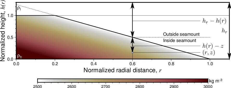
A linear density distribution selected with option -H. Flank density can be affected by water pressure if \(\Delta \rho_f > 0\), while the normalized internal density gradient is raised to power p to allow for nonlinear gradients. Note: The reference height H refers to a very tall seamount for which the supplied densities are suitable. Smaller seamounts will thus see lower core densities by virtue of being smaller.

-Kdensitymodel

Append the file name for a crossection grid with the predicted densities of the reference model. We use normalized coordinates (both x (radius) and y (height) go from 0 to 1 in increments of 0.005), yielding a fixed 201 x 201 grid. Note: This option can be used without creating the seamount grid, hence -R, -I, -G, and -D are not required.

-L[hn]

List area, volume, and mean height for each seamount; no grid will be created. Optionally, append hn for a noise-floor cutoff level below which we ignore area and volume [0].

-M[list]

Write the times and names of all relief grids (and density grids if -W is set) that were created to the text file list. Requires -T. If no list file is given then we write to standard output. The leading single numerical column will be time in years, while the last trailing text word is formatted time. The output listing is suitable as input to grdflexure. Note: The output records thus contain time reliefgrid [ densitygrid ] timetag.

-Nnorm

Normalize the relief grid(s) so the maximum grid height equals norm [no normalization].

-Qbmode[/fmode][+d]

Set build modes. Can only be used in conjunction with -T. The default is -Qc/g; append alternative mode settings (separated by a slash if both are specified) to change that:

• The required bmode determines how we construct the surface: Specify c for cumulative volume through time or i for the incremental volume added for each time increment.

• The optional fmode determines the volume flux curve we use: Give c for a constant volume flux or g for a Gaussian volume flux [Default] between the start and stop times of each feature.

These flux models integrate to a linear and error-function volume fraction curve over time, respectively, as shown below. By default, we compute the exact cumulative and incremental values for the seamounts specified. Append +d to instead approximate each incremental layer by a disc of constant thickness.

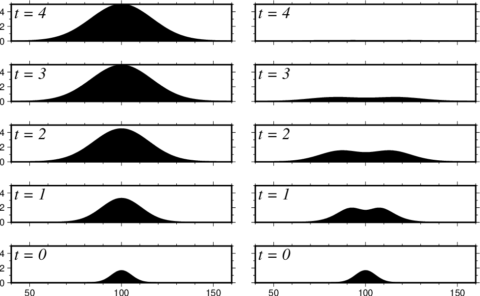
Use bmode in -Q to choose between cumulative output (c; actual topography as function of time [left]) or incremental output (i; the differences in actual topography over five time-steps [right]). Here, we used -Cg for a Gaussian model with no flattening and a Gaussian volume flux.

Use fmode in -Q to choose between a constant (c; dashed line) or Gaussian (g; heavy line) volume flux model. Note: We adjust the error-function curve so that it goes exactly from 0 to 1 over the time window.

-S[+a[az1/az2]][+b[beta]][+d[hc]][+h[h1/h2]][+p[power]][+t[t0/t1]][+u[u0]][+v[phi]]

Set parameters controlling the simulation of sectoral, rotational land slides by providing suitable modifiers. Parameters given on the command line apply to all seamounts equally. However, if a modifier is set but not given an argument then we read those arguments from the end of the input record; the order of such input arguments follows alphabetically from the modifier codes (and not the order the modifiers may appear on the command line). Repeat the slide group columns if there is more than one slide to read per seamount. Use these modifiers to set relevant slide parameters:

• +a specifies the azimuthal sector affected by the slide [0/360].

• +b sets a positive power coefficient \(\beta\) for the normalized slide volume fraction time-curve \(\psi(\tau) = \tau^\beta\) [Default is linear, i.e., 1]. See +t for definition of \(\tau\).

• +d sets the flank level of the seamount where the debris deposit begins [\(h_1/2\)].

• +h sets the lower and upper heights of the flank source area generating the landslide.

• +p activates angular variation in the radial slide profile; append a power parameter power > 2. Note: For multiple slides it is valid to provide power = 0 for some (either via command argument or read from file), which simply turns off angular variation for those slides. See +u for the radial slide profile setting.

• +t sets the time span over which the slide develops via \(\psi(\tau)\) (see +b), where \(\tau = (t - t_0)/(t_1 - t_0)\) is the normalized time span 0-1 when the slide occurs; this modifier also requires -T to be set.

• +u sets normalized radial slide shape parameter \(u_0 > 0\) [0.2].

• +v sets desired fractional volume \(\phi\) of the slide (in percent) relative to the entire seamount volume.

Note: If +v is set then we must compute the corresponding u0, hence +u is not allowed. If +b, +d, or +u are not set then their defaults are used for all slides. Currently, we support a maximum of 10 slides per seamount.

Geometry for an ad hoc landslide approximation (via cross-section modifiers +d and +h and map-view parameter +a). The volume of the slide material (pink) will be deposited at or below the toe of the surface rupture (light blue), starting at a height of \(h_c\) and linearly tapering to zero at a distal point \(r_d\). The various radii are computed from the heights and the shape function of the seamount. Note: \(h_2 > h_1\) while \(r_1 > r_2\).

-Tt0[/t1/dt][+l]

Specify t0, t1, and time increment (dt) for a sequence of calculations [Default is one step, with no time dependency]. For a single specific time, just give start time t0. Default unit is years; append k for kyr and M for Myr. For a logarithmic time scale, append +l and given the number of steps n instead of increment dt. Alternatively, give a file with the desired times in the first column (these times may have individual units appended, otherwise we assume year). If -T is set, then the input seamount table is expected to have to extra columns for the start and stop time following the initial seamount parameters (but before any slide groups; see -S). Because positive time is in years before present, we require t0 >= t1 time. Note: A grid will be written for all time-steps even if there are no relief or changes for one or more output times.

-V[level]

Select verbosity level [w]. (See full description) (See technical reference).

-Wavedensity

Give the name of the vertically averaged density grid file. If -T is set then avedensity must be a filename template (See File Template for details). Requires -H to define the density model.

-Zlevel

Set the background water depth [0]. As all seamounts have positive relief, you may use a larger negative level to place them under water. Alternatively, append NaN if you wish to flag unused nodes (not allowed if -Qi is used).

-birecord[+b|l] (more …)

Select native binary format for primary table input. [Default is 4 input columns].

-e[~]“pattern” | -e[~]/regexp/[i] (more …)

Only accept data records that match the given pattern.

-fflags

Geographic grids (dimensions of longitude, latitude) will be converted to km via a “Flat Earth” approximation using the current ellipsoid parameters.

-h[i|o][n][+c][+d][+msegheader][+rremark][+ttitle] (more …)

Skip or produce header record(s). Not used with binary data.

-icols[+l][+ddivisor][+sscale|d|k][+ooffset][,…][,t[word]] (more …)

Select input columns and transformations (0 is first column, t is trailing text, append word to read one word only).

-r[g|p] (more …)

Set node registration [gridline].

-:[i|o] (more …)

Swap 1st and 2nd column on input and/or output.

-^ or just -

Print a short message about the syntax of the command, then exit (Note: on Windows just use -).

-+ or just +

Print an extensive usage (help) message, including the explanation of any module-specific option (but not the GMT common options), then exit.

-? or no arguments

Print a complete usage (help) message, including the explanation of all options, then exit.

--PAR=value

Temporarily override a GMT default setting; repeatable. See gmt.conf for parameters.

Units

For map distance unit, append unit d for arc degree, m for arc minute, and s for arc second, or e for meter [Default unless stated otherwise], f for foot, k for km, M for statute mile, n for nautical mile, and u for US survey foot. By default we compute such distances using a spherical approximation with great circles (-jg) using the authalic radius (see PROJ_MEAN_RADIUS). You can use -jf to perform “Flat Earth” calculations (quicker but less accurate) or -je to perform exact geodesic calculations (slower but more accurate; see PROJ_GEODESIC for method used).

File Template

The format statements allowed in grid file templates require you to follow these rules:

• To use the formatted time-tag as part of the file name you must use just a single %s format as part of the template (e.g., smt_%s.grd).

• If you want to control the numerical formatting of the names but still have the common time unit appended then you must compose a template that has a floating point format before a later %c format for the unit. For example, smt_%05.1f%c.grd will create names like smt_001.1M.grd names. The times will be scaled to match the unit.

• If you do not want any units then simply give a template with just one floating point format, e.g., smt_%05.1f_name.grd. The times will be used as is (i.e, unscaled).

For details on the format statements, see printf C language format syntax.

Slide simulation specifics

The simulation of land slides via -S is not a physical model (apart from preserving mass). Instead, we approximate the shapes of rotational landslides and their evolution via simple geometric shapes and functions. The radial slide height is modeled as

\[h_s(r) = h_s(u) = h_1 + (h_2 - h_1)q(u) = h_1 + (h_2 - h_1) u_0 \left (\frac{1 + u_0}{u + u_0} - 1\right ),\]

where \(u = (r - r_2)/(r_1 - r_2)\) is the normalized horizontal distance of the rupture surface. This shape can be modulated by using +u to change \(u_0\).

A variety of normalized radial slide shapes \(q(u)\) is available by varying \(u_0\) (via modifier +u). For instance, the slide area for a conical seamount would be the area between the flank (dashed line) and the selected curve. A smaller \(u_0\) will cut more deeply into the seamount.

By default, the radial slide profile is fixed regardless of where in the slide sector we look. However, gentle or more abrupt angular variation can be added to \(h_s(r)\) via the function

\[s(\alpha) = s(\gamma) = 1 - \lvert \gamma \rvert ^p,\]

where \(\gamma = 2 (\alpha - \alpha_1)/(\alpha_2 - \alpha_1) - 1\) and p is the power exponent that can be set via +p. When enabled, we use \(s(\alpha)\) to scale the radial slide profile so that it starts of at zero at the two sectoral locations and then grows more (larger p) or less (smaller p) rapidly as we enter the slide sector. This modifier has the effect of smoothing the step functions we otherwise encounter as we enter the slide sector.

A range of azimuthal amplitude variation in radial slide height \(h_s(r)\) can be achieved by modulating the power parameter, p (via modifier +p). This variation means the slide volume is reduced by \(1 - \bar{s}\) (dashed lines). E.g., for p = 2 the slide volume is only 67% of the volume it would have been if there was no azimuthal variation (i.e., s = 1 [Default]).

Finally, an observed landslide may not have occurred instantly but developed over a finite time period. We can simulate that by distributing the total slide volume over this time. The normalized volume rate distribution is simulated by

\[\psi(t) = \psi(\tau) = \tau^\beta = \left (\frac{t - t_0}{t_1 - t_0} \right )^\beta,\]

where \(\tau\) is the normalized time during a slide event. We use this function to compute the portion of the slide volume that should be deposited at a given time t. Modifier +b is used to specify the power exponent \(\beta\) [1].

We can control how quickly a slide evolves over time by manipulating the \(\psi(\tau)\) function (via modifier +b). A linear curve means mass redistribution is taking place at a constant rate during the slide duration. Adjust \(\beta\) to have the bulk of the redistribution take place early (\(\beta < 1\)) or closer to the end (\(\beta > 1\)) of the event.

Notes

Because the Gaussian curve only drops to 1.11% of its peak amplitude at the base radius (3 sigma) of a seamount, we actually evaluate Gaussian curves all the way to 4 sigma so that the amplitude drops to 0.034% of peak height before we jump to zero. This prevents the otherwise very noticeable step at the base of the seamount.

Examples

To compute the shape of a circular Gaussian seamount located at 1W, 2S on a 1 arc minute grid for a basal radius of 30 km and a height of 4500 meters, try:

echo 1W 2S 30 4500 | gmt grdseamount -R1:30W/0:30W/2:30S/1:30S -I1m -Ggeo_circ_smt.nc
gmt grdimage geo_circ_smt.nc -B -png circ

To compute the shape of an elliptical conic seamount located at 200,400 on a 1x1 Cartesian grid for basal semi-major axis of 35 and semi-minor axis of 20, with an azimuth of 29 for the major axis, a height of 3700 meters, and some flattening (0.15), try:

echo 200 400 29 35 20 3700 | gmt grdseamount -R150/250/350/450 -I1 -E -F0.15 -Gcat_ell_smt.nc
gmt grdview cat_ell_smt.nc -B -Qi -I+d -JZ2c -p195/20 -png ell

To compute the incremental loads from two elliptical, truncated Gaussian seamounts being constructed from 3 Ma to 2 Ma and 2.8 M to 1.9 Ma using a constant volumetric production rate, and output an incremental grid every 0.1 Myr from 3 Ma to 1.9 Ma, and internally use meters for horizontal distances, we can try:

cat << EOF > t.txt
#lon lat azimuth, semi-major, semi-minor, height tstart tend
0   0       -20     120     60      5000    3.0M    2M
50  80      -40     110     50      4000    2.8M    21.9M
EOF
gmt grdseamount -R-1024/1022/-1122/924+uk -I2000 -Gsmt_%3.1f_%s.nc t.txt -T3M/1.9M/0.1M -Qi/c -Dk -E -F0.2 -Cg -Mfiles.txt

The file files.txt will contain records with numerical time, gridfile, and formatted-time.

Note: There are many more examples of use, including working with grdflexure, in the test directory for the potential supplement.

See Also

gmt.conf, gmt, grdmath, gravfft, grdflexure

Reference

Smith, J. R. and Wessel, P., 2000, Isostatic consequences of giant landslides on the Hawaiian Ridge, Pure Appl. Geophys., 157, 1097-1114, https://doi.org/10.1007/s000240050019.