The Global Self-consistent, Hierarchical, High-resolution Geography Database (GSHHG)

GMT uses the coast utility to access a version of the GSHHG data specially formatted for GMT. The GSHHG data have strengths and weaknesses. It is global and open source, but is based on relatively old datasets and hence may not be accurate enough for very large-scale mapping projects. The current GSHHG version used by GMT is 2.3.7. Below is a mostly technical description of how the GSHHG data set was assembled, processed, and formatted to meet the requirements of GMT.

Selecting the right data

There are two well-known public-domain data sets that could be used for this purpose. Once is known as the World Data Bank II or CIA Data Bank (WDB) and contains coastlines, lakes, political boundaries, and rivers. The other, the World Vector Shoreline (WVS) only contains shorelines between saltwater and land (i.e., no lakes). It turns out that the WVS data is far superior to the WDB data as far as data quality goes, but as noted it lacks lakes, not to mention rivers and borders. We decided to use the WVS whenever possible and supplement it with WDB data. We got these data over the Internet; they are also available on CD-ROM from the National Centers for Environmental Information in Boulder, Colorado [1].

Format required by GMT

In order to paint continents or oceans it is necessary that the coastline data be organized in polygons that may be filled. Simple line segments can be used to draw the coastline, but for painting polygons are required. Both the WVS and WDB data consists of unsorted line segments: there is no information included that tells you which segments belong to the same polygon (e.g., Australia should be one large polygon). In addition, polygons enclosing land must be differentiated from polygons enclosing lakes since they will need different paint. Finally, we want coast to be flexible enough that it can paint the land or the oceans or both. If just land (or oceans) is selected we do not want to paint those areas that are not land (or oceans) since previous plot programs may have drawn in those areas. Thus, we will need to combine polygons into new polygons that lend themselves to fill land (or oceans) only (Note that older versions of coast always painted lakes and wiped out whatever was plotted beneath).

The long and winding road

The WVS and WDB together represent more than 100 Mb of binary data and something like 20 million data points. Hence, it becomes obvious that any manipulation of these data must be automated. For instance, the reasonable requirement that no coastline should cross another coastline becomes a complicated processing step.

• To begin, we first made sure that all data were “clean”, i.e., that there were no outliers and bad points. We had to write several programs to ensure data consistency and remove “spikes” and bad points from the raw data. Also, crossing segments were automatically “trimmed” provided only a few points had to be deleted. A few hundred more complicated cases had to be examined semi-manually.

• Programs were written to examine all the loose segments and determine which segments should be joined to produce polygons. Because not all segments joined exactly (there were non-zero gaps between some segments) we had to find all possible combinations and choose the simplest combinations. The WVS segments joined to produce more than 200,000 polygons, the largest being the Africa-Eurasia polygon which has 1.4 million points. The WDB data resulted in a smaller data base (~25% of WVS).

• We now needed to combine the WVS and WDB data bases. The main problem here is that we have duplicates of polygons: most of the features in WVS are also in WDB. However, because the resolution of the data differ it is nontrivial to figure out which polygons in WDB to include and which ones to ignore. We used two techniques to address this problem. First, we looked for crossovers between all possible pairs of polygons. Because of the crossover processing in step 1 above we know that there are no remaining crossovers within WVS and WDB; thus any crossovers would be between WVS and WDB polygons. Crossovers could mean two things: (1) A slightly misplaced WDB polygon crosses a more accurate WVS polygon, both representing the same geographic feature, or (2) a misplaced WDB polygon (e.g., a small coastal lake) crosses the accurate WVS shoreline. We distinguished between these cases by comparing the area and centroid of the two polygons. In almost all cases it was obvious when we had duplicates; a few cases had to be checked manually. Second, on many occasions the WDB duplicate polygon did not cross its WVS counterpart but was either entirely inside or outside the WVS polygon. In those cases we relied on the area-centroid tests.

• While the largest polygons were easy to identify by visual inspection, the majority remain unidentified. Since it is important to know whether a polygon is a continent or a small pond inside an island inside a lake we wrote programs that would determine the hierarchical level of each polygon. Here, level = 1 represents ocean/land boundaries, 2 is land/lakes borders, 3 is lakes/islands-in-lakes, and 4 is islands-in-lakes/ponds-in-islands-in-lakes. Level 4 was the highest level encountered in the data. To automatically determine the hierarchical levels we wrote programs that would compare all possible pairs of polygons and find how many polygons a given polygon was inside. Because of the size and number of the polygons such programs would typically run for 3 days on a Sparc-2 workstation.

• Once we know what type a polygon is we can enforce a common “orientation” for all polygons. We arranged them so that when you move along a polygon from beginning to end, your left hand is pointing toward “land”. At this step we also computed the area of all polygons since we would like the option to plot only features that are bigger than a minimum area to be specified by the user.

• Obviously, if you need to make a map of Denmark then you do not want to read the entire 1.4 million points making up the Africa-Eurasia polygon. Furthermore, most plotting devices will not let you paint and fill a polygon of that size due to memory restrictions. Hence, we need to partition the polygons so that smaller subsets can be accessed rapidly. Likewise, if you want to plot a world map on a letter-size paper there is no need to plot 10 million data points as most of them will plot several times on the same pixel and the operation would take a very long time to complete. We chose to make 5 versions on the database, corresponding to different resolutions. The decimation was carried out using the Douglas-Peucker (DP) line-reduction algorithm [2]. We chose the cutoffs so that each subset was approximately 20% the size of the next higher resolution. The five resolutions are called full, high, intermediate, low, and crude; they are accessed in coast, gmtselect, and grdlandmask with the -D option [3]. For each of these 5 data sets (f, h, i, l, c) we specified an equidistant grid (1, 2, 5, 10, 20) and split all polygons into line-segments that each fit inside one of the many boxes defined by these grid lines. Thus, to paint the entire continent of Australia we instead paint many smaller polygons made up of these line segments and gridlines. Some book-keeping has to be done since we need to know which parent polygon these smaller pieces came from in order to prescribe the correct paint or ignore if the feature is smaller than the cutoff specified by the user. The resulting segment coordinates were then scaled to fit in short integer format to preserve precision and written in netCDF format for ultimate portability across hardware platforms [4].

• While we are now back to a file of line-segments we are in a much better position to create smaller polygons for painting. Two problems must be overcome to correctly paint an area:

  • We must be able to join line segments and grid cell borders into meaningful polygons; how we do this will depend on whether we want to paint the land or the oceans.
  • We want to nest the polygons so that no paint falls on areas that are “wet” (or “dry”); e.g., if a grid cell completely on land contains a lake with a small island, we do not want to paint the lake and then draw the island, but paint the annulus or “donut” that is represented by the land and lake, and then plot the island.

  GMT uses a polygon-assembly routine that carries out these tasks on the fly.

The Five Resolutions

We will demonstrate the power of the new database by starting with a regional hemisphere map centered near Papua New Guinea and zoom in on a specified point. The map regions will be specified in projected km from the projection center, e.g., we may want the map to go from km to km in the longitudinal and the latitudinal direction. Also, as we zoom in on the projection center we want to draw the outline of the next map region on the plot. To do that we use the -D option in basemap.

The crude resolution (-Dc)

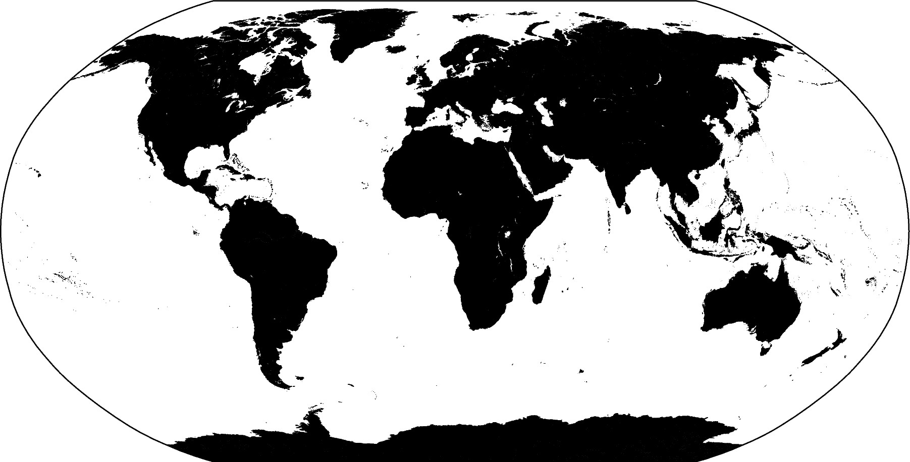
We begin with an azimuthal equidistant map of the hemisphere centered on 130°21’E, 0°12’S, which is slightly west of New Guinea, near the Strait of Dampier. The edges of the map are all 9000 km true distance from the projection center. At this scale (and for global maps) the crude resolution data will usually be adequate to capture the main geographic features. To avoid cluttering the map with insignificant detail we only plot features (i.e., polygons) that exceed 500 km² in area. Smaller features would only occupy a few pixels on the plot and make the map look “dirty”. We also add national borders to the plot. The crude database is heavily decimated and simplified by the DP-routine: The total file size of the coastlines, rivers, and borders database is only 283 kbytes. The plot is produced by the script:

gmt begin GMT_App_K_1
  gmt set MAP_GRID_CROSS_SIZE_PRIMARY 0 MAP_ANNOT_OBLIQUE 22 MAP_ANNOT_MIN_SPACING 0.3i
  gmt coast -Rk-9000/9000/-9000/9000 -JE130.35/-0.2/3.5i -Dc \
    -A500 -Gburlywood -Sazure -Wthinnest -N1/thinnest,- -B20g20 -BWSne
  echo 130.35 -0.2 | gmt plot -SJ-4000 -Wthicker
gmt end show

Map using the crude resolution coastline data.

Here, we use the MAP_ANNOT_OBLIQUE bit flags to achieve horizontal annotations and set MAP_ANNOT_MIN_SPACING to suppress some longitudinal annotations near the S pole that otherwise would overprint. The square box indicates the outline of the next map.

The low resolution (-Dl)

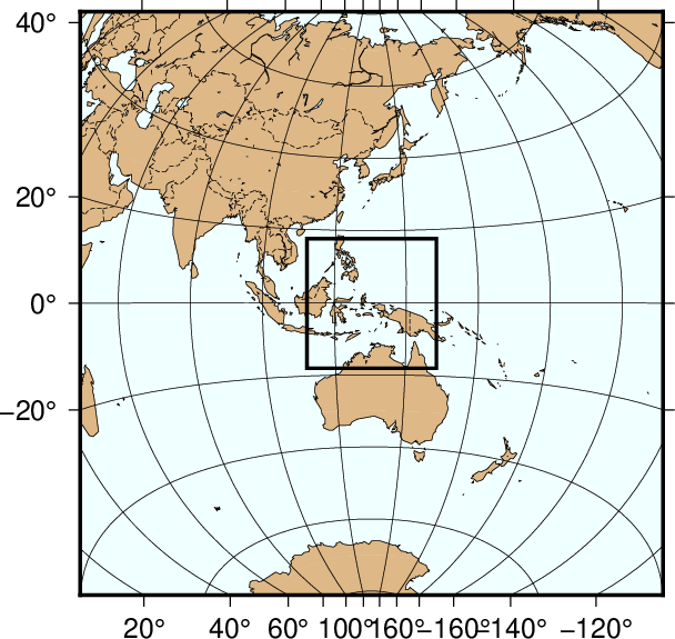
We have now reduced the map area by zooming in on the map center. Now, the edges of the map are all 2000 km true distance from the projection center. At this scale we choose the low resolution data that faithfully reproduce the dominant geographic features in the region. We cut back on minor features less than 100 km² in area. We still add national borders to the plot. The low database is less decimated and simplified by the DP-routine: The total file size of the coastlines, rivers, and borders combined grows to 907 kbytes; it is the default resolution in GMT. The plot is generated by the script:

gmt begin GMT_App_K_2
  gmt coast -Rk-2000/2000/-2000/2000 -JE130.35/-0.2/3.5i -Dl -A100 -Gburlywood -Sazure -Wthinnest -N1/thinnest,- -B10g5 -BWSne
  echo 130.35 -0.2 | gmt plot -SJ-1000 -Wthicker
gmt end show

Map using the low resolution coastline data.

The intermediate resolution (-Di)

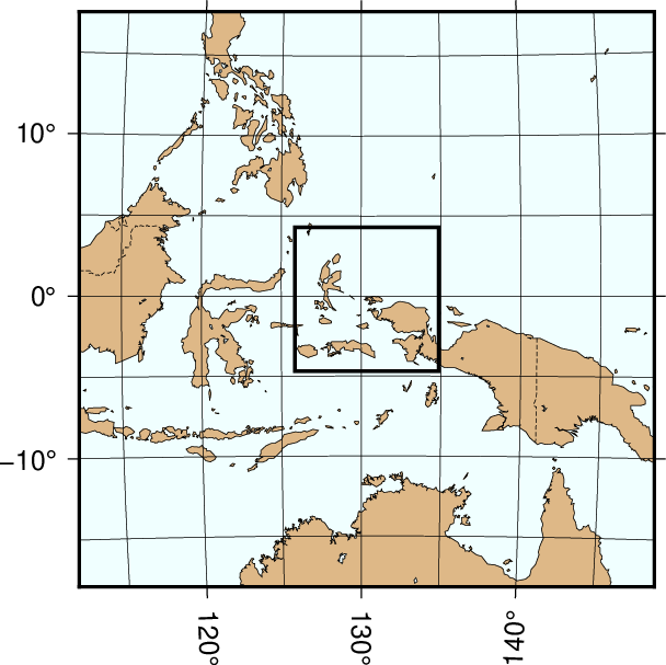
We continue to zoom in on the map center. In this map, the edges of the map are all 500 km true distance from the projection center. We abandon the low resolution data set as it would look too jagged at this scale and instead employ the intermediate resolution data that faithfully reproduce the dominant geographic features in the region. This time, we ignore features less than 20 km² in area. Although the script still asks for national borders none exist within our region. The intermediate database is moderately decimated and simplified by the DP-routine: The combined file size of the coastlines, rivers, and borders now exceeds 3.35 Mbytes. The plot is generated by the script:

gmt begin GMT_App_K_3
  gmt coast -Rk-500/500/-500/500 -JE130.35/-0.2/3.5i -Di -A20 \
    -Gburlywood -Sazure -Wthinnest -N1/thinnest,- -B2g1 -BWSne
  echo 133 2 | gmt plot -Sc1.4i -Gwhite
  gmt basemap -Tm133/2+w1i+t45/10/5+jCM --FONT_TITLE=12p --MAP_TICK_LENGTH_PRIMARY=0.05i \
    --FONT_ANNOT_SECONDARY=8p
  echo 130.35 -0.2 | gmt plot -SJ-200 -Wthicker
gmt end show

Map using the intermediate resolution coastline data. We have added a compass rose just because we have the power to do so.

The high resolution (-Dh)

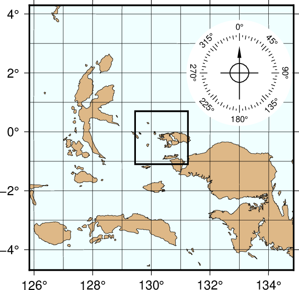
The relentless zooming continues! Now, the edges of the map are all 100 km true distance from the projection center. We step up to the high resolution data set as it is needed to accurately portray the detailed geographic features within the region. Because of the small scale we only ignore features less than 1 km² in area. The high resolution database has undergone minor decimation and simplification by the DP-routine: The combined file size of the coastlines, rivers, and borders now swells to 12.3 Mbytes. The map and the final outline box are generated by these commands:

gmt begin GMT_App_K_4
  gmt coast -Rk-100/100/-100/100 -JE130.35/-0.2/3.5i -Dh -A1 \
    -Gburlywood -Sazure -Wthinnest -N1/thinnest,- -B30mg10m -BWSne
  echo 130.35 -0.2 | gmt plot -SJ-40 -Wthicker
gmt end show

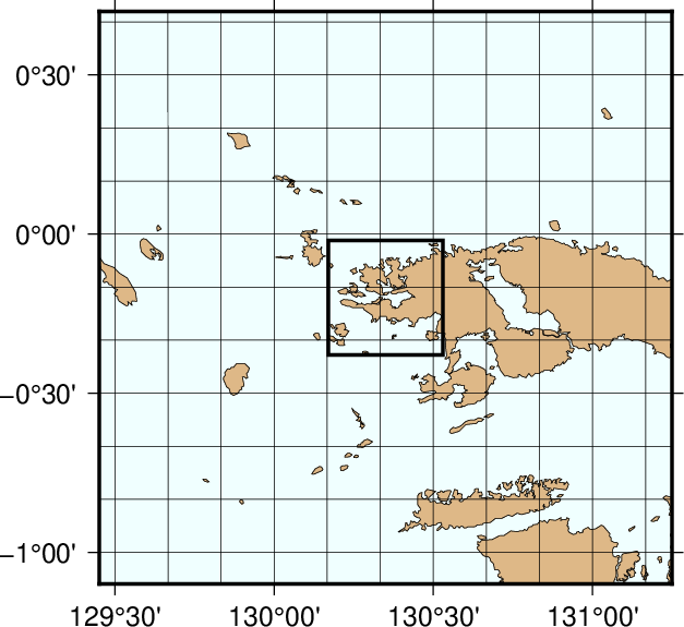
Map using the high resolution coastline data.

The full resolution (-Df)

We now arrive at our final plot, which shows a detailed view of the western side of the small island of Waigeo. The map area is approximately 40 by 40 km. We call upon the full resolution data set to portray the richness of geographic detail within this region; no features are ignored. The full resolution has undergone no decimation and it shows: The combined file size of the coastlines, rivers, and borders totals a (once considered hefty) 55.9 Mbytes. Our final map is reproduced by the single command:

gmt coast -Rk-20/20/-20/20 -JE130.35/-0.2/3.5i -Df -Gburlywood \
            -Sazure -Wthinnest -N1/thinnest,- -B10mg2m -BWSne -pdf GMT_App_K_5

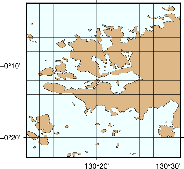
Map using the full resolution coastline data.

We hope you will study these examples to enable you to make efficient and wise use of this vast data set.

[1]	National Centers for Environmental Information, Boulder, Colorado

[2]	Douglas, D.H., and T. K. Peucker, 1973, Algorithms for the reduction of the number of points required to represent a digitized line or its caricature, Canadian Cartographer, 10, 112–122.

[3]	The full and high resolution files are in separate archives because of their size. Not all users may need these files as the intermediate data set is better than the data provided with version 2.2.4.

[4]	If you need complete polygons in a simpler format, see the article on GSHHG (Wessel, P., and W. H. F. Smith, 1996, A Global, self-consistent, hierarchical, high-resolution shoreline database, J. Geophys. Res. 101, 8741–8743).