1. The Generic Mapping Tools
Technical Reference and Cookbook
Pål (Paul) Wessel
SOEST, University of Hawai’i at Manoa
Walter H. F. Smith
Laboratory for Satellite Altimetry, NOAA/NESDIS/STAR
Remko Scharroo
EUMETSAT, Darmstadt, Germany
Joaquim F. Luis
Universidade do Algarve, Faro, Portugal
Florian Wobbe
Alfred Wegener Institute, Germany
The five horsemen of the GMT apocalypse: Joaquim Luis, Walter H.F. Smith, Remko Scharroo, Florian Wobbe, and Paul Wessel at the GMT Developer Summit in La Jolla, Cailifornia, during August 15--19, 2016.
1.1. Acknowledgments
The Generic Mapping Tools (GMT) could not have been designed without
the generous support of several people. The Founders (Wessel and Smith)
gratefully acknowledge A. B.
Watts and the late W. F. Haxby for supporting their efforts on the
original version 1.0 while they were their graduate students at
Lamont-Doherty Earth Observatory. Doug Shearer and Roger Davis patiently
answered many questions over e-mail. The subroutine gauss was
written and supplied by Bill Menke. Further development of versions
2.0--2.1 at SOEST would not have been possible without the support from
the HIGP/SOEST Post-Doctoral Fellowship program to Paul Wessel. Walter
H. F. Smith gratefully acknowledges the generous support of the C. H.
and I. M. Green Foundation for Earth Sciences at the Institute of
Geophysics and Planetary Physics, Scripps Institution of Oceanography,
University of California at San Diego. GMT series 3.x, 4.x, and 5.x
owe their existence to grants EAR-93-02272, OCE-95-29431, OCE-00-82552,
OCE-04-52126, and OCE-1029874 from the National Science Foundation,
which we gratefully acknowledge.
We would also like to acknowledge feedback, suggestions and bug reports from Michael Barck, Manfred Brands, Allen Cogbill, Stephan Eickschen, Ben Horner-Johnson, John Kuhn, Angel Li, Andrew Macrae, Alex Madon, Ken McLean, Greg Neumann, Ameet Raval, Georg Schwarz, Richard Signell, Peter Schmidt, Dirk Stoecker, Eduardo Suárez, Mikhail Tchernychev, Malte Thoma, David Townsend, Garry Vaughan, William Weibel, and many others, including their advice on how to make GMT portable to a wide range of platforms. John Lillibridge and Stephan Eickschen provided the original Examples (11) and (32), respectively; Hanno von Lom helped resolve early problems with DLL libraries for Win32; Lloyd Parkes enabled indexed color images in PostScript; Kurt Schwehr maintains the packages; Wayne Wilson implemented the full general perspective projection; and William Yip helped translate GMT to POSIX ANSI C and incorporate netCDF 3. The SOEST RCF staff (Ross Ishida, Pat Townsend, and Sharon Stahl) provided valuable help on Linux and web server support.
Honolulu, HI; College Park, MD; Faro, Portugal; Darmstadt and Bremerhaven, Germany; September 2016
2. A Reminder
If you feel it is appropriate, you may consider paying us back by citing our EOS articles on GMT and technical papers on algorithms when you publish papers containing results or illustrations obtained using GMT. The EOS articles on GMT are
- Wessel, P., W. H. F. Smith, R. Scharroo, J. Luis, and F. Wobbe, Generic Mapping Tools: Improved Version Released, EOS Trans. AGU, 94(45), p. 409-410, 2013. doi:10.1002/2013EO450001.
- Wessel, P., and W. H. F. Smith, New, improved version of Generic Mapping Tools released, EOS Trans. AGU, 79(47), p. 579, 1998. doi:10.1029/98EO00426.
- Wessel, P., and W. H. F. Smith, New version of the Generic Mapping Tools released, EOS Trans. AGU, 76(33), 329, 1995. doi:10.1029/95EO00198.
- Wessel, P., and W. H. F. Smith, Free software helps map and display data, EOS Trans. AGU, 72(41), 445--446, 1991. doi:10.1029/90EO00319.
Some GMT modules are based on algorithms we have developed and published separately, such as
- Kim, S.-S., and P. Wessel, Directional median filtering for regional-residual separation of bathymetry, Geochem. Geophys. Geosyst., 9, Q03005, 2008. doi:10.1029/2007GC001850. [dimfilter, misc supplement]
- Luis, J. F. and J. M. Miranda, Reevaluation of magnetic chrons in the North Atlantic between 35ºN and 47ºN: Implications for the formation of the Azores Triple Junction and associated plateau, J. Geophys. Res., 113, B10105, 2008. doi:10.1029/2007JB005573. [grdredpol, potential supplement]
- Smith, W. H. F., and P. Wessel, Gridding with continuous curvature splines in tension, Geophysics, 55(3), 293--305, 1990. doi:10.1190/1.1442837. [surface]
- Wessel, P., Tools for analyzing intersecting tracks: The x2sys package, Computers & Geosciences, 36, 348--354, 2010. doi:10.1016/j.cageo.2009.05.009. [x2sys supplement]
- Wessel, P., A General-purpose Green’s function-based interpolator, Computers & Geosciences, 35, 1247--1254, 2009. doi:10.1016/j.cageo.2008.08.012. [greenspline]
- Wessel, P. and J. M. Becker, Interpolation using a generalized Green’s function for a spherical surface spline in tension, Geophys. J. Int., 174, 21--28, 2008. doi:10.1111/j.1365-246X.2008.03829.x. [greenspline]
Finally, GMT includes some code supplied by others, in particular the Triangle code used for Delaunay triangulation. Its author, Jonathan Shewchuk, says
“If you use Triangle, and especially if you use it to accomplish real work, I would like very much to hear from you. A short letter or email describing how you use Triangle will mean a lot to me. The more people I know are using this program, the more easily I can justify spending time on improvements and on the three-dimensional successor to Triangle, which in turn will benefit you.”
A few GMT users take the time to write us letters, telling us of the difference GMT is making in their work. We appreciate receiving these letters. On days when we wonder why we ever released GMT we pull these letters out and read them. Seriously, as financial support for GMT depends on how well we can “sell” the idea to funding agencies and our superiors, letter-writing is one area where GMT users can affect such decisions by supporting the GMT project.
3. Copyright and Caveat Emptor!
Copyright ©1991--2019 by P. Wessel, W. H. F. Smith, R. Scharroo, J. Luis and F. Wobbe
The Generic Mapping Tools (GMT) is free software; you can redistribute it and/or modify it under the terms of the GNU Lesser General Public License as published by the Free Software Foundation.
The GMT package is distributed in the hope that it will be useful,
but WITHOUT ANY WARRANTY; without even the implied warranty of
MERCHANTABILITY or FITNESS FOR A PARTICULAR PURPOSE. See the file
LICENSE.TXT in the GMT directory or the for more details.
Permission is granted to make and distribute verbatim copies of this manual provided that the copyright notice and these paragraphs are preserved on all copies. The GMT package may be included in a bundled distribution of software for which a reasonable fee may be charged.
GMT does not come with any warranties, nor is it guaranteed to work on your computer. The user assumes full responsibility for the use of this system. In particular, the University of Hawaii School of Ocean and Earth Science and Technology, the National Oceanic and Atmospheric Administration, EUMETSAT, the Universidade do Algarve, Alfred Wegener Institute, the National Science Foundation, Paul Wessel, Walter H. F. Smith, Remko Scharroo, Joaquim F. Luis, Florian Wobbe or any other individuals involved in the design and maintenance of GMT are NOT responsible for any damage that may follow from correct or incorrect use of these programs.
4. Preface
While GMT has served the map-making and data processing needs of
scientists since 1988 [1], the current global use was heralded by the
first official release in EOS Trans. AGU in the fall of 1991. Since
then, GMT has grown to become a standard tool for many users,
particularly in the Earth and Ocean Sciences but the global collective
of GMT users is incredibly diverse. Development has at times been
rapid, and numerous releases have seen the light of day since the early
versions. For a detailed history of the changes from release to release,
see file ChangeLog in the main GMT directory. For a nightly snapshot of ongoing
activity, see the online page. For a historical perspective of the
origins and development of GMT see the video podcast “20 Years with
GMT -- The Generic Mapping Tools” produced following a seminar given by
Paul Wessel on the 20th anniversary of GMT; a link is available on the
GMT website.
The success of GMT is to a large degree due to the input of the user community. In fact, most of the capabilities and options in the GMT modules originated as user requests. We would like to hear from you should you have any suggestions for future enhancements and modification. Please send your comments to the GMT help list or create an issue in the bug tracker (see http://gmt.soest.hawaii.edu/projects/gmt/issues/).
5. New Features in GMT 5.4
Between 5.3 and 5.4 we continued to work on the underlying API needed to support the modules and especially the external interfaces we are building toward MATLAB, Julia and Python. We have introduced the use of static analyzers to fix any code irregularities and we continue to submit our builds to Coverity for similar reasons. We have also made an effort to standardize GMT non-common option usage across the suite. Nevertheless, there have been many user-level enhancements as well. Here is a summary of these changes in three key areas:
5.1. New modules
We have added a new module to the GMT core called psternary. This module allows for the construction of ternary diagram, currently restricted to symbols (i.e., a psxy-like experience but for ternary data). The mgd77 supplement has gained a new tool mgd77header for creating a valid MGD77-format header from basic metadata and information determined from the header-less data file.
5.2. General improvements
A range of new capabilities have been added to all of GMT; here is a summary of these changes:
- We have added a new lower-case GMT common option. Programs that read ASCII data can use -e to only select data records that match a specified pattern or regular expression.
- All modules can now read data via external URL addresses. This works by using libcurl to access an external file and save it to the users’ GMT cache directory. This directory can be specified via a new GMT defaults called DIR_CACHE (and defaults to the sub-directory cache under the $GMT_USERDIR directory [~/.gmt]). Subsequent use of the same URL will be read from the cache (except if explicitly removed by the user). An exception is CGI Get Commands which will be executed anew each time. Both the user directory and the cache directory will be created if they do not exist.
- Any reference to Earth topographic/bathymetric relief files called earth_relief_res.grd will automatically obtain the grid from the GMT data server. The resolution res allows a choice among 13 command grid spacings: 60m, 30m, 20m, 15m, 10m, 6m, 5m, 4m, 3m, 2m, 1m, 30s, and 15s (with file sizes 111 kb, 376 kb, 782 kb, 1.3 Mb, 2.8 Mb, 7.5 Mb, 11 Mb, 16 Mb, 27 Mb, 58 Mb, 214 Mb, 778 Mb, and 2.6 Gb respectively). Once one of these have been downloaded any future reference will simply obtain the file from $GMT_USERDIR (except if explicitly removed by the user).
- We are laying the groundwork for more dynamic documentation. At present, the examples on the man pages (with the exception of psbasemap and pscoast) cannot be run by cut and paste since they reference imaginary data sets. These will soon appear with filenames starting in @ (e.g., @hotspots.txt), and when such files are found on the command line it is interpreted to be a shorthand notation for the full URL to the GMT cache data server.
- We have added four new color tables inspired by matplotlib to the collection. These CPTs are called plasma, magma, inferno, and viridis.
- We have updated the online documentation of user-contributed custom symbols and restored the beautiful biological symbols for whales and dolphins created by Pablo Valdés during the GMT4 era. These are now complemented by new custom symbols for structural geology designed by José A. Álvarez-Gómez.
- The PSL library no longer needs run-time files to configure the list of standard fonts and character encodings, reducing the number of configure files required.
- The gmt.conf files produced by gmt set will only write parameters that differ from the GMT SI Standard settings. This means most gmt.conf files will just be a few lines.
- We have deprecated the -ccopies option whose purpose was to modify the number of copies a printer would issue give a PostScript file. This is better controlled by your printer driver and most users now work with PDF files.
- The -p option can now do a simple rotation about the z-axis (i.e., not a perspective view) for more advanced plotting.
- The placement of color scales around a map can now be near-automatic, as the -DJ setting now has many default values (such as for bar length, width, offsets and orientation) based on which side you specified. If you use this option in concert with -B to turn off frame annotation on the side you place the scale bar then justification works exactly.
- The -i option to select input columns can now handle repeat entries, e.g., -i0,2,2,4, which is useful when a column is needed as a coordinate and for symbol color or size.
- The vector specifications now take one more modifier: +hshape allows vectors to quickly set the head shape normally specified via MAP_VECTOR_SHAPE. This is particularly useful when the symbol types are given via the input file.
- The custom symbol macro language has been strengthened and now allows all angular quantities to be variables (i.e., provided from your data file as extra columns), the pen thickness can be specified as relative (and thus scale with the symbol size at run-time), and a symbol can internally switch colors between the pen and fill colors given on the command line.
- We have reintroduced the old GMT4 polygon-vector for those who fell so hard in love with that symbol. By giving old-style vector specifications you will now get the old-style symbol. The new and superior vector symbols will require the use of the new (and standard) syntax.
5.3. Module enhancements
Several modules have obtained new options to extend their capabilities:
- gmt has new session management option that lets you clear various files and cache directories via the new commands gmt clear all|history|conf|cache.
- gmt2kml adds option -Fw for drawing wiggles along track.
- gmtinfo adds option -F for reporting the number of tables, segments, records, headers, etc.
- gmtmath will convert all plot dimensions given on the command line to the prevailing length unit set via PROJ_LENGTH_UNIT. This allows you to combine measurements like 12c, 4i, and 72p. The module also has a new SORT operator for sorting columns and RMSW for weighted root-mean-square.
- gmtwhich -G will download a file from the internet (as discussed above) before reporting the path to the file (which will then be in the user’s cache directory).
- grd2xyz can now write weights equal to the area each node represents via the -Wa option.
- grdgradient can now take a grid of azimuths via the -A option.
- grdimage and grdview can now auto-compute the intensities directly from the required input grid via -I, and this option now supports modifiers +a and +n for changing the options of the grdgradient call within the module.
- grdinfo adds option -D to determine the regions of all the smaller-size grid tiles required to cover the larger area. It also take a new argument -Ii for reporting the exact region of an img grid. Finally, we now report area-weighted statistics for geographic grids, added -Lp for mode (maximum-likelihood) estimate of location and scale, and -La for requesting all of the statistical estimates.
- grdmath has new operators TRIM, which will set all grid values that fall in the specified tails of the data distribution to NaN, NODE, which will create a grid with node indices 0 to (nx*ny)-1, and RMSW, which will compute the weighted root-mean-square.
- makecpt and grd2cpt add option -Ws for producing wrapped (cyclic) CPT tables that repeat endlessly. New CPT keyword CYCLIC controls if the CPT is cyclic.
- mapproject adds a new -Z option for temporal calculations based on distances and speeds, and has been redesigned to allow several outputs by combining the options -A, -G, -L, and -Z.
- psbasemap has a new map-insert (-D) modifier +t that will translate the plot origin after determining the lower-left corner of the map insert.
- pshistogram has a new -Z modifier +w that will accumulate weights provided in the 2nd input column instead of pure counts.
- psrose adds option -Q for setting the confidence level used for a Rayleigh test for uniformity of direction. The -C option also takes a new modifier +wmodfile for storing mode direction to file.
- gmt_shell_functions.sh adds numerous new functions to simplify the building of animation scripts, animated GIF and MP4 videos, launching groups of jobs across many cores, packaging KMLs into a single KMZ archive, and more.
5.4. API changes
We have introduced one change that breaks backwards compatibility for users of the API functions. We don’t do this lightly but given the API is still considered beta it was the best solution. Function GMT_Create_Data now requires the mode to be GMT_IS_OUTPUT (an new constant) if a dummy (empty) container should be created to hold the output of a module. We also added two new API functions GMT_Duplicate_Options and GMT_Free_Option to manage option lists, and added the new constants GMT_GRID_IS_CARTESIAN and GMT_GRID_IS_GEO so that external tools can communicate the nature of grid written in situations where there are no projections involved (hence GMT does not know a grid is geographic). Passing this constant will be required in MB-System.
5.5. Backwards-compatible syntax changes
We strive to keep the GMT user interface consistent. The common options help with that, but the module-specific options have often used very different forms to achieve similar goals. We have revised the syntax of numerous options across the modules to use the common modifier method. However, as no GMT users would be happy that their scripts no longer run, these changes are backwards compatible. Only the new syntax will be documented but old syntax will be accepted. Some options are used across GMT and will get a special mention first:
- Many modules use -G to specify the fill (solid color or pattern). The pattern specification has now changed to be -Gp|Ppattern[+bcolor][+fcolor][+rdpi]
- When specifying grids one can always add information such as grid type, scaling, offset, etc. This is now done using a cleaner syntax for grids: gridfile[=ID[+sscale][+ooffset][+ninvalid]].
Here is a list of modules with revised options:
- grdcontour now expects -Z[+scale][+ooffset][+p].
- In grdedit and xyz2grd, the mechanism to change a grid’s metadata is now done via modifiers to the -D option, such as +xxname, +ttitle, etc.
- grdfft has changed to -E[+w[k]][+n].
- grdgradient modifies the syntax of -E and -N by introducing modifiers, i.e., -E[m|s|p]azim/elev[+aambient][+ddiffuse][+pspecular][+sshine] and -N[e|t][amp][+ssigma][+ooffset].
- grdtrend follows trend1d and now wants -Nmodel[+r].
- mapproject introduces new and consistent syntax for -G and -L as -G[lon0/lat0][+a][+i][+u[+|-]unit][+v] and -Lline.xy[+u[+|-]unit][+p].
- project expects -Ginc[/lat][+h].
- psrose now wants -L[wlabel,elabel,slabel,nlabel] to match the other labeling options.
- pstext now expects -D[j|J]dx[/dy][+v[pen]].
- psxy expects -E[x|y|X|Y][+a][+cl|f][+n][+wcap][+ppen].
- trend2d follows trend1d and now wants -Nmodel[+r].
6. New Features in GMT 5.3
Between 5.2 and 5.3 we spent much time working on the underlying API needed to support the modules and especially the external interfaces we are building toward MATLAB and Python. Nevertheless, there have been many user-level enhancements as well. Here is a summary of these changes in three key areas:
6.1. New modules
We have added a new module to the GMT core called pssolar. This module plots various day-light terminators and other sunlight parameters.
Two new modules have been added to the spotter supplement: The first is gmtpmodeler. Like grdpmodeler it evaluates plate tectonic model predictions but at given point locations locations instead of on a grid. The second is rotsmoother which smooths estimated rotations using quaternions.
Also, the meca supplement has gained a new tool pssac for the plotting of seismograms in SAC format.
Finally, we have added gpsgridder to the potential supplement. This tool is a Green’s function gridding module that grids vector data assumed to be coupled via an elastic model. The prime usage is for gridding GPS velocity components.
6.2. General improvements
There are many changes to GMT, mostly under the hood, but also changes that affect users directly. We have added four new examples and one new animation to highlight recently added capabilities. There have been many bug fixes as well. For specific enhancements, we have:
- All GMT-distributed color palette tables (CPTs, now a total of 44) are dynamic and many have a hinge and a default range. What this means is that the range of all CPTs have been normalized to 0-1, expect that those with a hinge are normalized to -1/+1, with 0 being the normalized hinge location. CPTs with a hinge are interpolated separately on either side of the hinge, since a hinge typically signifies a dramatic color change (e.g., at sea-level) and we do not want that color change to be shifted to some other z-value when an asymmetrical range is being requested. In situations where no range is specified then some CPTs will have a default range and that will be substituted instead. The tools makecpt and grd2cpt now displays more meta-data about the various CPTs, including values for hinge, range, and the color-model used.
- We have consolidated how map embellishments are specified. This group includes map scales, color bars, legends, map roses, map inserts, image overlays, the GMT logo, and a background panel. A new section in the Cookbook is dedicated to these items and how they are specified. Common to all is the concept of a reference point relative to which the item is justified and offset.
- We continue to extend support for OpenMP in GMT. New modules that are OpenMP-enabled are grdgradient, grdlandmask, and sph2grd.
- blockmean, blockmedian and blockmode have a new modifier +s to the -W option. When used we expect 1-sigma uncertainties instead of weights and compute weight = 1/sigma.
- filter1d: can now compute high-pass filtered output via a new +h modifier to the filter settings, similar to existing capability in grdfilter.
- gmtconvert has a new option (-F) for line segmentation and network configuration. Also, the -D option has a new modifier +o that sets the origin used for the numbering of tables and segments.
- gmtinfo has a new option -L for finding the common bounds across multiple files or segments. Also, the -T option has been modified (while still being backwards compatible) to allow dz to be optional, with modifiers +s forcing a symmetric range and +a offering alpha-trimming of the tails before estimating the range.
- gmtmath has gained new operators VAR, RMS, DENAN, as well as the weighted statistical operators LMSSCLW, MADW, MEANW, MEDIANW, MODEW, PQUANTW, STDW, and VARW. Finally, we added a SORT operator that lets you sort an entire table in ascending or descending order based on the values in a selected column.
- gmtselect has a new option -G for selecting based on a mask grid. Points falling in bins whose grid nodes are non-zero are selected (or not if -Ig)
- gmtspatial has two new modifiers for the -Q option that allow output segments to be limited based on the segment length (or area for polygons) as well as sorting the output in ascending or descending order.
- grd2cpt existing -F option now takes a new modifier +c for writing a discrete palette using the categorical format.
- grdedit can now reset text items in the header via -D by specifying ‘-‘. Also, new -C option can be used to reset the command history in the header.
- grdfft has a new modifier to the -E option that allows for more control of the power normalization for radial spectra.
- grdmath also has the new operators VAR, RMS, DENAN, as well as the weighted statistical operators LMSSCLW, MADW, MEANW, MEDIANW, MODEW, PQUANTW, STDW, and VARW. In addition it gains a new AREA operator which computes the gridcell area (in km2 if the grid is geographic). Finally, operators MEAN, MEDIAN, etc., when working on a geographic grid, will weight the result using the AREA function for proper spherical statistics.
- grdvolume can now accept -Crcval which will evaluate the volume between cval and the grid’s minimum value.
- greenspline now offers a new -E option that evaluates the model fit at the input data locations and optionally saves the model misfits to a secondary output file.
- makecpt can also let you build either a discrete or continuous custom color palette table from a comma-separated list of colors and z-values provided via a file, an equidistant setup, or comma-separated list. The -F option now takes a new modifier +c for writing a discrete palette using the categorical format.
- pstext has new modifiers to its -F option that allows users to generate automatic labels such as record numbers of formatting of a third data column into a textual representation. We also allow any baseline angles to be interpreted as orientations, i.e., they will be modified to fall in the -90/+90 range when -F…+A is set.
- psrose can now control the attributes of vectors in a windrose diagram via -M.
- psxy have seen numerous enhancements. New features include decorated lines, which are similar to quoted lines except we place symbols rather than text along the line. Users also gain new controls over the plotting of lines, including the ability to add vector heads to the line endings, to trim back lines by specified amounts, and to request a Bezier spline interpolation in PostScript (see enhanced -W option). A new option (-F) for line segmentation and networks have also been added. Various geographic symbols (such as ellipses; -SE, rotatable rectangles -SJ; and geo-vectors -S=) can now take size in geographic dimensions, including a new geo-wedge symbol. We also offer one more type of fault-slip symbol, using curved arrow heads. Also the arrow head selections now include inward-pointing arrows. Custom symbols may now simply be a preexisting EPS figure. Many of these enhancements are also available in psxyz.
- The spotter supplement now comes with the latest rotation files from EarthByte, U. of Sydney.
6.3. The API
We have spend most of our time strengthening the API, in particular in support of the GMT/MATLAB toolbox. A few new API functions have been added since the initial release, including GMT_Get_Pixel, GMT_Set_Index, GMT_Open_VirtualFile, GMT_Close_VirtualFile, GMT_Read_VirtualFile, GMT_Read_Group, and GMT_Convert_Data; see the API Introduction for details.
7. New Features in GMT 5.2
While the GMT 5.1-series has seen bug-fixes since its release, new features were only added to the 5.2-series. All in all, almost 200 new features (a combination of new programs, new options, and enhancements) have been implemented. Here is a summary of these changes in six key areas:
7.1. New modules
There are two new modules in the core system:
gmtlogo is modeled after the shell script with the same name but is now a regular C module that can be used to add the GMT logo to maps and posters.
gmtregress determines linear regressions for data sets using a variety of misfit norms and regression modes.
Four new modules have also been added to the potential supplement:
- gmtflexure:
- Compute the elastic flexural response to a 2-D (line) load.
- grdflexure:
- Compute the flexural response to a 3-D (grid) load, using a variety or rheological models (elastic, viscoelastic, firmoviscous).
- talwani2d:
- Compute a profile of the free-air gravity, geoid or vertical gravity gradient anomaly over a 2-D body given as cross-sectional polygons.
- talwani3d:
- Compute a grid or profile of the free-air gravity, geoid or vertical gravity gradient anomaly over a 3-D body given as horizontal polygonal slices.
In addition, two established modules have been given more suitable names (however, the old names are still recognized):
- grdconvert
- Converts between different grid formats. Previously known as grdreformat (this name is recognized when GMT is running in compatibility mode).
- psconvert
- Converts from PostScript to PDF, SVG, or various raster image formats. Previously known as ps2raster (this name is recognized when GMT is running in compatibility mode).
Finally, we have renamed our PostScript Light (PSL) library from psl to PostScriptLight to avoid package name conflicts. This library will eventually become decoupled from GMT and end up as a required prerequisite.
7.2. New common options
We have added two new lower-case GMT common options:
- Programs that need to specify which values should represent “no data” can now use -d[i|o]nodata. For instance, this option replaces the old -N in grd2xyz and xyz2grd (but is backwards compatible).
- Some modules are now using OpenMP to spread computations over all available cores (only available if compiled with OpenMP support). Those modules will offer the new option -x[[-]n] to reduce how many cores to assign to the task. The modules that currently have this option are greenspline, grdmask, grdmath, grdfilter, grdsample, sph2grd, the potential supplement’s grdgravmag3d, talwani2d and talwani3d, and the x2sys supplement’s x2sys_solve. This list will grow longer with time.
7.3. New default parameters
There have been a few changes to the GMT Defaults parameters. All changes are backwards compatible:
- FORMAT_FLOAT_MAP now allows the use %’g to get comma-separated groupings when integer values are plotted.
- FORMAT_FLOAT_OUT can now accept a space-separated list of formats as shorthand for first few columns. On output it will show the formats in effect for multiple columns.
- GMT_LANGUAGE has replaced the old parameter TIME_LANGUAGE. Related to this, the files share/time/*.d have been moved and renamed to share/localization/*.txt and now include a new section or cardinal points letter codes.
- IO_SEGMENT_BINARY is a new parameter that controls how binary records with just NaNs should or should not be interpreted as segment headers.
- PROJ_GEODESIC was added to control which geodesic calculation should be used. Choose among Vincenty [Default], Andoyer (fast approximate geodesics), and Rudoe (from GMT4).
- TIME_REPORT now has defaults for absolute or elapsed time stamps.
7.4. Updated common options
Two of the established GMT common options have seen minor improvements:
- Implemented modifier -B+n to not draw the frame at all.
- Allow oblique Mercator projections to select projection poles in the southern hemisphere by using upper-case selectors A|B|C.
- Added a forth way to specify the region for a new grid via the new -R[L|C|R][T|M|B]x0/y0/nx/ny syntax where you specify an reference point and number of points in the two dimensions (requires -I to use the increments). The optional justification keys specify how the reference point relate to the grid region.
7.5. General improvements
Several changes have affects across GMT; these are:
- Added optional multi-threading capabilities to several modules, such as greenspline, grdfilter, grdmask, grdsample, the potential supplement’s grdgravmag3d, talwani2d and talwani3d and x2sys’s x2sys_solve.
- Optional prerequisite LAPACK means SVD decomposition in greenspline is now very fast, as is true for the regular Gauss-Jordan solution via a new multi-processor enabled algorithm.
- Allow comma-separated colors instead of CPTs in options that are used to pass a CPT (typically this means the -C option).
- Faster netCDF reading for COARDS table data (i.e., not grids).
- When importing grids via GDAL the projection info is preserved and stored as netCDF metadata. This will allow third party programs like GDAL and QGIS to recognize the projection info of GMT created grids. Same thing happens when creating grids with grdproject.
- Tools using GSHHG can now access information for both Antarctica data sets (ice-front and grounding line).
- Tools that specify pens may now explicitly choose “solid” as an attribute, and we added “dashed” and “dotted” as alternatives to the shorthands “-” and “.”.
- Added three alternative vector head choices (terminal, square and circle) in addition to the default “arrow” style. We have also added the option for trimming the beginning and/or end point location of a vector, and you may now place the vector head at the mid-point of the vector instead at the ends.
- All eight map embellishment features (map scale, color bar, direction rose, magnetic rose, GMT logo, raster images, map inserts, and map legends) now use a uniform mechanism for specifying placement, justification, and attributes and is supported by a new section in the documentation.
- Typesetting simultaneous sub- and super-scripts has improved (i.e., when a symbol should have both a subscript and and a superscript).
- The custom symbol macro codes now allow for an unspecified symbol code (?), which means the desired code will be given as last item on each data record. Such custom symbols must be specified with uppercase -SK.
7.6. Program-specific improvements
Finally, here is a list of enhancements to individual modules. Any changes to existing syntax will be backwards compatible:
- fitcircle now has a new option -F that allows output to be in the form of coordinates only (no text report) and you may choose which items to return by appending suitable flags.
- gmt now has a --show-cores option that reports the available cores.
- gmtconvert adds a -C option that can be used to eliminate segments on output based on the number of records it contains. We also added a -F option to create line segments from an input data sets using a variety of connectivity modes.
- gmtmath adds a long list of new operators. We have the operator BPDF for binomial probability distribution and BCDF for the cumulative binomial distribution function. Due to confusion with other probability distributions we have introduced a series of new operator names (but honor backwards compatibility). Listing the pdf and cdf for each distribution, these are TPDF and TCDF for the Student t-distribution, FPDF and FCDF for the F-distribution, CHI2PDF and CHI2CDF for the Chi-squared distribution, EPDF and ECDF for the exponential distribution (as well as ECRIT), PPDF and PCDF for the Poisson distribution, LPDF and LCDF for the Laplace distribution (as well as LCRIT), RPDF and RCDF for the Rayleigh distribution (as well as RCRIT), WPDF and WCDF for the Weibull distribution (as well as WCRIT), and ZPDF and ZCDF for the Normal distribution. We added ROLL for cyclic shifts of the stack, and DENAN as a more intuitive operator for removing NaNs, as well as new constants TRANGE, TROW, F_EPS and D_EPS, and we have renamed the normalized coordinates from Tn to TNORM (but this is backwards compatible). We added operator POINT which reads a data table and places the mean x and mean y on the stack. Finally, we added new hyperbolic and inverse hyperbolic functions COTH and ACOTH, SECH and ASECH, and CSCH and ACSCH.
- gmtspatial now lets you specify Flat Earth or Geodesic distance calculations for line lengths via -Q.
- grdblend relaxes the -W restriction on only one output grid and adds the new mode -Wz to write the weight*zsum grid.
- grdedit enhances the -E option to allow for 90-degree rotations or flips of grid, as well as a new -G to enable writing of the result to a new output file [Default updates the existing file]. The -J option saves the georeferencing info as metadata in netCDF grids.
- grdfilter now includes histogram mode filtering to complement mode (LMS) filtering.
- grdgradient adds -Da to compute the aspect (down-slope) direction [up-slope].
- grdinfo reports the projection info of netCDF grids when that is stored in a grid’s metadata in WKT format.
- grdmath adds numerous new operators, such as ARC and WRAP for angular operators, BPDF for binomial probability distribution and BCDF for the cumulative binomial distribution function. Due to confusion with other probability distributions we have introduced a series of new operator names (but accept backwards compatibility). Listing the pdf and cdf for each distribution, these are TPDF and TCDF for the Student t-distribution, FPDF and FCDF for the F-distribution, CHI2PDF and CHI2CDF for the Chi-squared distribution, EPDF and ECDF for the exponential distribution (as well as ECRIT), PPDF and PCDF for the Poisson distribution, LPDF and LCDF for the Laplace distribution (as well as LCRIT), RPDF and RCDF for the Rayleigh distribution (as well as RCRIT), WPDF and WCDF for the Weibull distribution (as well as WCRIT), and ZPDF and ZCDF for the Normal distribution. We added LDISTG (for distances to GSHHG), CDIST2 and SDIST2 (to complement LDIST2 and PDIST2), and ROLL for cyclic shifts of the stack, and DENAN as a more intuitive operator for removing NaNs, while LDIST1 has been renamed to LDISTC. We also add new constants XRANGE, YRANGE, XCOL, YROW and F_EPS, and we have renamed the normalized coordinates from Xn to XNORM and Yn to YNORM (but this is backwards compatible). Finally, we added new hyperbolic and inverse hyperbolic functions COTH and ACOTH, SECH and ASECH, and CSCH and ACSCH.
- grdtrack add the modifier -G+llist to pass a list of grids.
- grdview implements the Waterfall plot mode via -Qmx|y.
- kml2gmt acquires a -F option to control which geometry to output.
- makecpt takes -E to determine range from an input data table.
- mapproject can be used in conjunction with the 3-D projection options to compute 3-D projected coordinates. We also added -W to simply output the projected dimensions of the plot without reading input data.
- psbasemap now takes -A to save the plot domain polygon in geographical coordinates. The -L option for map scale and -T for map roses have been revised (backwards compatible) and a new uniform -F option to specify background panel and its many settings was added.
- pscoast can accept multiple -E settings to color several features independently. We also have the modifiers +AS to only plot Antarctica, +ag to use shelf ice grounding line for Antarctica coastline, and +ai to use ice/water front for Antarctica coastline [Default]. As above, the -L option for map scale and -T option for map roses have been revised (backwards compatible) and a new uniform -F option to specify background panel and its many settings was added.
- psconvert (apart from the name change) has several new features, such as reporting dimensions of the plot when -A and -V are used, scaling the output plots via -A+s[m]width[u][/height[u]], paint and outline the bounding box via -A modifiers gfill and +ppen, and -Z for removing the PostScript file on exit. In addition, we have added SVG as a new output vector graphics format and now handle transparency even if non-PDF output formats are requested.
- pscontour adds a -Qcut option like grdcontour and consolidates the old -T, -Q options for an index file to a new -E option.
- pshistogram added modifiers -Wwidth[+l|h|b] to allow for more control on what happens to points falling in the tails.
- psimage added a new uniform -D option to specify location of the image and new uniform -F option to specify background panel and its many settings.
- pslegend has many enhancements for specifying varying cell widths and color, as well as a new uniform -D option to specify location of legend and new uniform -F option to specify background panel and its many settings.
- psscale new uniform -D option to specify location of the scale. We have retired the -T option in favor of the new uniform -F option to specify background panel and its many settings.
- psxy has seen considerable enhancements. We added two new quoted line (-Sq) modifiers: S|s for treating input as consecutive two-point line segments that should be individually quoted, and +x[first,last] for automating cross-section labeling. We added a new symbol (-S~) for decorated lines. These are very similar to quoted lines but instead place specified symbols along lines. We expanded -N to handle periodic, repeating symbols near the boundary, added a new modifier + to -E for asymmetrical error bars, and provided the shorthand -SE-diameter for degenerated ellipses (i.e., circles). The -L option has been enhanced to create envelope polygons around y(x), say for confidence envelopes (modifiers +b|d|D), and to complete a closed polygon by adding selected corners (modifiers +xl|r|x0 or +yb|t|y0). The -A-option now has new modifiers x|y for creating stair-case curves. The slip-vector symbol can now optionally accept a vector-head angle [30]. The custom symbols definition tests can now compare two input variables. We also added a -F option to draw line segments from an input data sets using a variety of connectivity modes. Finally, for drawing lines there are new line attribute modifiers available via the pen setting -W such as drawing with a Bezier spline (+s), trimming the segments from the ends before plotting (+ooffset), or adding vector heads at the ends of the lines (+v).
- psxyz also has the new -SE-diameter shorthand as well as the -N modifiers for handling periodic plot symbols. Like, psxy it gets the same improvements to quoted lines and adds decorated lines as a new symbol. Likewise, the -L option has been enhanced to create envelope polygons around y(x), say for confidence envelopes (modifiers +b|d|D), and to complete a closed polygon by adding selected corners (modifiers +xl|r|x0 or +yb|t|y0). The slip-vector symbol can now optionally accept a vector-head angle [30]. Finally, to match psxy we have added the option -T for specifying no data input.
- sample1d spline selection option -F can now accept the optional modifiers +1 or +2 which will compute the first or second derivatives of the spline, respectively.
- spectrum1d can now turn off single-output data to stdout via -T or turn off multi-file output via -N.
- sphdistance can now also perform a nearest-neighbor gridding where all grid nodes inside a Voronoi polygon is set to the same value as the Voronoi node value, via -Ez.
- trend1d can now fit mixed polynomial and Fourier series models, as well as allowing models with just some terms in a polynomial or a Fourier series, including plain cosine or sine series terms. Modifiers have been added to specify data origin and fundamental period instead of defaulting to the data mid-point and data range, respectively.
A few supplement modules have new features as well:
- mgd77track adds the -Gngap option to decimate the trackline coordinates by only plotting every gap point.
- gravfft adds -Wwd to change observation level.
- grdgravmag3d adds -H to compute magnetic anomaly.
- grdpmodeler can now output more than one model prediction into several grids or as a record written to stdout. Also gains the -N option used by other spotter tools to extend the model duration.
8. New Features in GMT 5
GMT 5 represents a new branch of GMT development that mostly preserves the
capabilities of the previous versions while adding over 200 new features
to an already extensive bag of tricks. Our PostScript library
PSL has seen a complete rewrite as well
and produce shorter and more compact PostScript. However, the big news
is aimed for developers who wish to leverage GMT in their own applications.
We have completely revamped the code base so that high-level
GMT functionality is now accessible via GMT “modules”. These are
high-level functions named after their corresponding programs (e.g.,
GMT_grdimage) that contains all of the functionality of that program
within the function. While currently callable from C/C++ only (with some
support for F77), we are making progress on the Matlab interface as well
and there are plans to start on the Python version. Developers should
consult the GMT API documentation for more details.
We recommend that users of GMT 4 consider learning the new rules and defaults since eventually (in some years) GMT 4 will be obsolete. To ease the transition to GMT 5 you may run it in compatibility mode, thus allowing the use of many obsolete default names and command switches (you will receive a warning instead). This is discussed below.
Below are six key areas of improvements in GMT 5.
8.1. New programs
First, a few new programs have been added and some have been promoted (and possibly renamed) from earlier supplements:
- gmt
- This is the only program executable that is distributed with GMT 5. To avoid problems with namespace conflicts (e.g., there are other, non-GMT programs with generic names like triangulate, surface, etc.) all GMT 5 modules are launched from the gmt executable via “gmt module” calls (e.g, gmt pscoast). For backwards compatibility (see below) we also offer symbolic links with the old executable names that simply point to the gmt program, which then can start the correct module. Any module whose name starts with “gmt” can be abbreviated, e.g., “gmt gmtconvert” may be called as “gmt convert”.
- gmt2kml
- A psxy -like tool to produce KML overlays for Google Earth. Previously found in the misc supplement.
- gmtconnect
- Connect individual lines whose end points match within given tolerance. Previously known as gmtstitch in the misc supplement (this name is recognized when GMT is running in compatibility mode).
- gmtget
- Return the values of the specified GMT defaults. Previously only implemented as a shell script and thus not available on all platforms.
- gmtinfo
- Report information about data tables. Previously known by the name minmax (this name is still recognized when GMT is running in compatibility mode).
- gmtsimplify
- A line-reduction tool for coastlines and similar lines. Previously found in the misc supplement under the name gmtdp (this name is recognized when GMT is running in compatibility mode).
- gmtspatial
- Perform various geospatial operations on lines and polygons.
- gmtvector
- Perform basic vector manipulation in 2-D and 3-D.
- gmtwhich
- Return the full path to specified data files.
- grdraster
- Extracts subsets from large global grids. Previously found in the dbase supplement.
- kml2gmt
- Extract GMT data tables from Google Earth KML files. Previously found in the misc supplement.
- sph2grd
- Compute grid from list of spherical harmonic coefficients [We will add its natural complement grd2sph at a later date].
- sphdistance
- Make grid of distances to nearest points on a sphere. Previously found in the sph supplement.
- sphinterpolate
- Spherical gridding in tension of data on a sphere. Previously found in the sph supplement.
- sphtriangulate
- Delaunay or Voronoi construction of spherical lon,lat data. Previously found in the sph supplement.
We have also added a new supplement called potential that contains these five modules:
- gmtgravmag3d:
- Compute the gravity/magnetic anomaly of a body by the method of Okabe.
- gmtflexure:
- Compute the flexure of a 2-D load using variable plate thickness and restoring force.
- gravfft:
- Compute gravitational attraction of 3-D surfaces and a little more by the method of Parker.
- grdgravmag3d:
- Computes the gravity effect of one (or two) grids by the method of Okabe.
- grdredpol:
- Compute the Continuous Reduction To the Pole, also known as differential RTP.
- grdseamount:
- Compute synthetic seamount (Gaussian or cone, circular or elliptical) bathymetry.
Finally, the spotter supplement has added one new module:
- grdpmodeler:
- Evaluate a plate model on a geographic grid.
8.2. New common options
First we discuss changes that have been implemented by a series of new lower-case GMT common options:
- Programs that read data tables can now process the aspatial metadata in OGR/GMT files with the new -a option. These can be produced by ogr2ogr (a GDAL tool) when selecting the -f “GMT” output format. See Chapter The GMT Vector Data Format for OGR Compatibility for an explanation of the OGR/GMT file format. Because all GIS information is encoded via GMT comment lines these files can also be used in GMT 4 (the GIS metadata is simply skipped).
- Programs that read or write data tables can specify a custom binary format using the enhanced -b option.
- Programs that read data tables can control which columns to read and in what order (and optionally supply scaling relations) with the new -i option
- Programs that read grids can use new common option -n to control grid interpolation settings and boundary conditions.
- Programs that write data tables can control which columns to write and in what order (and optionally supply scaling relations) with the new -o option.
- All plot programs can take a new -p option for perspective view from infinity. In GMT 4, only some programs could do this (e.g., pscoast) and it took a program-specific option, typically -E and sometimes an option -Z would be needed as well. This information is now all passed via -p and applies across all GMT plotting programs.
- Programs that read data tables can control how records with NaNs are handled with the new -s option.
- All plot programs can take a new -t option to modify the PDF transparency level for that layer. However, as PostScript has no provision for transparency you can only see the effect if you convert it to PDF.
8.3. Updated common options
Some of the established GMT common options have seen significant improvements; these include:
- The completely revised -B option can now handle irregular and custom annotations (see Section Custom axes). It also has a new automatic mode which will select optimal intervals given data range and plot size. The 3-D base maps can now have horizontal gridlines on xz and yz back walls.
- The -R option may now accept a leading unit which implies the given coordinates are projected map coordinates and should be replaced with the corresponding geographic coordinates given the specified map projection. For linear projections such units imply a simple unit conversion for the given coordinates (e.g., km to meter).
- Introduced -fp[unit] which allows data input to be in projected values, e.g., UTM coordinates while -Ju is given.
While just giving - (the hyphen) as argument presents just the synopsis of the command line arguments, we now also support giving + which in addition will list the explanations for all options that are not among the GMT common set.
8.4. New default parameters
Most of the GMT default parameters have changed names in order to group parameters into logical groups and to use more consistent naming. However, under compatibility mode (see below) the old names are still recognized. New capabilities have been implemented by introducing new GMT default settings:
- DIR_DCW specifies where to look for the optional Digital Charts of the World database (for country coloring or selections).
- DIR_GSHHG specifies where to look for the required Global Self-consistent Hierarchical High-resolution Geography database.
- GMT_COMPATIBILITY can be set to 4 to allow backwards compatibility with GMT 4 command-line syntax or 5 to impose strict GMT5 syntax checking.
- IO_NC4_CHUNK_SIZE is used to set the default chunk size for the lat and lon dimension of the z variable of netCDF version 4 files.
- IO_NC4_DEFLATION_LEVEL is used to set the compression level for netCDF4 files upon output.
- IO_SEGMENT_MARKER can be used to change the character that GMT uses to identify new segment header records [>].
- MAP_ANNOT_ORTHO controls whether axes annotations for Cartesian plots are horizontal or orthogonal to the individual axes.
- GMT_FFT controls which algorithms to use for Fourier transforms.
- GMT_TRIANGULATE controls which algorithm to use for Delaunay triangulation.
- Great circle distance approximations can now be fine-tuned via new GMT default parameters PROJ_MEAN_RADIUS and PROJ_AUX_LATITUDE. Geodesics are now even more accurate by using the Vincenty [1975] algorithm instead of Rudoe’s method.
- GMT_EXTRAPOLATE_VAL controls what splines should do if requested to extrapolate beyond the given data domain.
- PS_TRANSPARENCY allows users to modify how transparency will be processed when converted to PDF [Normal].
A few parameters have been introduced in GMT 5 in the past and have been removed again. Among these are:
- DIR_USER: was supposed to set the directory in which the user configuration files, or data are stored, but this creates problems, because it needs to be known already before it is potentially set in DIR_USER/gmt.conf. The environment variable $GMT_USERDIR is used for this instead.
- DIR_TMP: was supposed to indicate the directory in which to store temporary files. But needs to be known without gmt.conf file as well. So the environment variable $GMT_TMPDIR is used instead.
8.5. General improvements
Other wide-ranging changes have been implemented in different ways, such as
- All programs now use consistent, standardized choices for plot dimension units (cm, inch, or point; we no longer consider meter a plot length unit), and actual distances (choose spherical arc lengths in degree, minute, and second [was c], or distances in meter [Default], foot [new], km, Mile [was sometimes i or m], nautical mile, and survey foot [new]).
- Programs that read data tables can now process multi-segment tables automatically. This means programs that did not have this capability (e.g., filter1d) can now all operate on the segments separately; consequently, there is no longer a -m option.
- While we support the scaling of z-values in grids via the filename convention name[=ID[+sscale][+ooffset][+nnan] mechanism, there are times when we wish to scale the x,y domain as well. Users can now append +uunit to their gridfile names, where unit is one of non-arc units listed in Table distunits. This will convert your Cartesian x and y coordinates from the given unit to meters. We also support the inverse option +Uunit, which can be used to convert your grid coordinates from meters to the specified unit.
- CPTs also support the +u|Uunit mechanism. Here, the scaling applies to the z values. By appending these modifiers to your CPT names you can avoid having two CPTs (one for meter and one for km) since only one is needed.
- Programs that read grids can now directly handle Arc/Info float binary files (GRIDFLOAT) and ESRI .hdr formats.
- Programs that read grids now set boundary conditions to aid further processing. If a subset then the boundary conditions are taken from the surrounding grid values.
- All text can now optionally be filled with patterns and/or drawn with outline pens. In the past, only pstext could plot outline fonts via -Spen. Now, any text can be an outline text by manipulating the corresponding FONT defaults (e.g., FONT_TITLE).
- All color or fill specifications may append @transparency to change the PDF transparency level for that item. See -t for limitations on how to visualize this transparency.
- GMT now ships with 36 standard color palette tables (CPT), up from 24.
8.6. Program-specific improvements
Finally, here is a list of numerous enhancements to individual programs:
- blockmean added -Ep for error propagation and -Sn to report the number of data points per block.
- blockmedian added -Er[-] to return as last column the record number that gave the median value. For ties, we return the record number of the higher data value unless -Er- is given (return lower). Added -Es to read and output source id for median value.
- blockmode added -Er[-] but for modal value. Added -Es to read and output source id for modal value.
- gmtconvert now has optional PCRE (regular expression) support, as well as a new option to select a subset of segments specified by segment running numbers (-Q) and improved options to extract a subset of records (-E) and support for a list of search strings via -S+fpatternfile.
- gmtinfo has new option -A to select what group to report on (all input, per file, or per segment). Also, use -If to report an extended region optimized for fastest results in FFTs. and -Is to report an extended region optimized for fastest results in surface. Finally, new option -D[inc] to align regions found via -I with the center of the data.
- gmtmath with -Nncol and input files will add extra blank columns, if needed. A new option -E sets the minimum eigenvalue used by operators LSQFIT and SVDFIT. Option -L applies operators on a per-segment basis instead of accumulating operations across the entire file. Many new operators have been added (BITAND, BITLEFT, BITNOT, BITOR, BITRIGHT, BITTEST, BITXOR, DIFF, IFELSE, ISFINITE, SVDFIT, TAPER). Finally, we have implemented user macros for long or commonly used expressions, as well as ability to store and recall using named variables.
- gmtselect Takes -E to indicate if points exactly on a polygon boundary are inside or outside, and -Z can now be extended to apply to other columns than the third.
- grd2cpt takes -F to specify output color model and -G to truncate incoming CPT to be limited to a given range.
- grd2xyz takes -C to write row, col instead of x,y. Append f to start at 1, else start at 0. Alternatively, use -Ci to write just the two columns index and z, where index is the 1-D indexing that GMT uses when referring to grid nodes.
- grdblend can now take list of grids on the command line and blend, and now has more blend choices (see -C). Grids no longer have to have same registration or spacing.
- grdclip has new option -Si to set all data >= low and <= high to the between value, and -Sr to set all data == old to the new value.
- grdcontour can specify a single contour with -C+contour and -A+contour.
- grdcut can use -S to specify an origin and radius and cut the corresponding rectangular area, and -N to extend the region if the new -R domain exceeds existing boundaries.
- grdfft can now accept two grids and let -E compute the cross-spectra. The -N option allows for many new and special settings, including ability to control data mirroring, detrending, tapering, and output of intermediate results.
- grdfilter can now do spherical filtering (with wrap around longitudes and over poles) for non-global grids. We have also begun implementing Open MP threads to speed up calculations on multi-core machines. We have added rectangular filtering and automatic resampling to input resolution for high-pass filters. There is also -Ffweightgrd which reads the gridfile weightgrd for a custom Cartesian grid convolution. The weightgrd must have odd dimensions. Similarly added -Foopgrd for operators (via coefficients in the grdfile opgrd) whose weight sum is zero (hence we do not sum and divide the convolution by the weight sum).
- grdgradient now has -Em that gives results close to ESRI’s “hillshade”’” (but faster).
- grdinfo now has modifier -Tsdz which returns a symmetrical range about zero. Also, if -Ib is given then the grid’s bounding box polygon is written.
- grdimage with GDAL support can write a raster image directly to a raster file (-A) and may plot raster images as well (-Dr). It also automatically assigns a color table if none is given and can use any of the 36 GMT color tables and scale them to fit the grid range.
- grdmask has new option -Ni|I|p|P to set inside of polygons to the polygon IDs. These may come from OGR aspatial values, segment head -LID, or a running number, starting at a specified origin [0]. Now correctly handles polygons with perimeters and holes. Added z as possible radius value in -S which means read radii from 3rd input column.
- grdmath added many new operators such as BITAND, BITLEFT, BITNOT, BITOR, BITRIGHT, BITTEST, BITXOR, DEG2KM, IFELSE, ISFINITE, KM2DEG, and TAPER. Finally, we have implemented user macros for long or commonly used expressions, as well as ability to store and recall using named variables.
- grdtrack has many new options. The -A option controls how the input track is resampled when -C is selected, the new -C, -D options automatically create an equidistant set of cross-sectional profiles given input line segments; one or more grids can then be sampled at these locations. The -E option allows users to quickly specify tracks for sampling without needed input tracks. Also added -S which stack cross-profiles generated with -C. The -N will not skip points that are outside the grid domain but return NaN as sampled value. Finally, -T will return the nearest non-NaN node if the initial location only finds a NaN value.
- grdvector can now take -Siscale to give the reciprocal scale, i.e., cm/ unit or km/unit. Also, the vector heads in GMT have completely been overhauled and includes geo-vector heads that follow great or small circles.
- grdview will automatically assigns a color table if none is given and can use any of the 36 GMT color tables and scale them to fit the grid range.
- grdvolume can let -S accept more distance units than just km. It also has a modified -T[c|h] for ORS estimates based on max curvature or height. -Cr to compute the outside volume between two contours (for instances, the volume of water from a bathymetry grid).
- greenspline has an improved -C option to control how many eigenvalues are used in the fitting, and -Sl adds a linear (or bilinear) spline.
- makecpt has a new -F option to specify output color representation, e.g., to output the CPT in h-s-v format despite originally being given in r/g/b, and -G to truncate incoming CPT to be limited to a given range. It also adds Di to match the bottom/top values in the input CPT.
- mapproject has a new -N option to do geodetic/geocentric conversions; it combines with -I for inverse conversions. Also, we have extended -A to accept -Ao| O to compute line orientations (-90/90). In -G, prepend - to the unit for (fast) flat Earth or + for (slow) geodesic calculations.
- project has added -G…[+] so if + is appended we get a segment header with information about the pole for the circle. Optionally, append /colat in -G for a small circle path.
- psconvert has added a -TF option to create multi-page PDF files. There is also modification to -A to add user-specified margins, and it automatically detects if transparent elements have been included (and a detour via PDF might be needed).
- psbasemap has added a -D option to place a map-insert box.
- psclip has added an extended -C option to close different types of clip paths.
- pscoast has added a new option -E which lets users specify one or more countries to paint, fill, extract, or use as plot domain (requires DCW to be installed).
- pscontour is now similar to grdcontour in the options it takes, e.g., -C in particular. In GMT 4, the program could only read a CPT and not take a specific contour interval.
- pshistogram now takes -D to place histogram count labels on top of each bar and -N to draw the equivalent normal distributions.
- pslegend no longer uses system calls to do the plotting. The modified -D allows for minor offsets, while -F offers more control over the frame and fill.
- psrose has added -Wvpen to specify pen for vector (specified in -C). Added -Zu to set all radii to unity (i.e., for analysis of angles only).
- psscale has a new option -T that paints a rectangle behind the color bar. The +n modifier to -E draws a rectangle with NaN color and adds a label. The -G option will truncate incoming CPT to be limited to the specified z-range. Modification -Np indicates a preference to use polygons to draw the color bar.
- pstext can take simplified input via new option -F to set fixed font (including size), angle, and justification. If these parameters are fixed for all the text strings then the input can simply be x y text. It also has enhanced -DJ option to shorten diagonal offsets by \(\sqrt{2}\) to maintain the same radial distance from point to annotation. Change all text to upper or lower case with -Q.
- psxy and psxyz both support the revised custom symbol macro language which has been expanded considerably to allow for complicated, multi-parameter symbols; see Chapter Custom Plot Symbols for details. Finally, we allow the base for bars and columns optionally to be read from data file by not specifying the base value.
- sample1d offers -A to control resampling of spatial curves (with -I).
- spectrum1d has added -L to control removal of trend, mean value or mid value.
- surface has added -r to create pixel-registered grids and knows about periodicity in longitude (given -fg). There is also -D to supply a “sort” break line.
- triangulate now offers -S to write triangle polygons and can handle 2-column input if -Z is given. Can also write triangle edges as line with -M.
- xyz2grd now also offers -Af (first value encountered), -Am (mean, the default), -Ar (rms), and -As (last value encountered).
Several supplements have new features as well:
- img2grd used to be a shell script but is now a C program and can be used on all platforms.
- mgd77convert added -C option to assemble *.mgd77 files from *.h77/*.a77 pairs.
- The spotter programs can now read GPlates rotation files directly as well as write this format. Also, rotconverter can extract plate circuit rotations on-the-fly from the GPlates rotation file.
Note: GMT 5 only produces PostScript and no longer has a setting for Encapsulated PostScript (EPS). We made this decision since (a) our EPS determination was always very approximate (no consideration of font metrics, etc.) and quite often wrong, and (b) psconvert handles it exactly. Hence, users who need EPS plots should simply process their PostScript files via psconvert.
8.7. Command-line completion
GMT provides basic command-line completion (tab completion) for bash. The easiest way to use the feature is to install the bash-completion package which is available in many operating system distributions.
Depending on the distribution, you may still need to source it from
~/.bashrc, e.g.:
# Use bash-completion, if available
if [ -r /usr/share/bash-completion/bash_completion ]; then
  . /usr/share/bash-completion/bash_completion
fi
When you install GMT from a distribution package, the completion rules
are installed in /etc/bash_completion.d/gmt and loaded automatically.
Custom GMT builds provide <prefix>/share/tools/gmt_completion.bash
which needs to be manually sourced from either ~/.bash_completion or
~/.bashrc.
Mac users should note that bash-completion >=2.0 requires bash >=4.1. However, OS X won’t ship anything that’s licensed under GPL version 3. The last version of bash available under the GPLv2 is 3.2 from 2006. It is recommended that bash-completion is installed together with bash via MacPorts, Fink, or Homebrew. You then need to change the shell used by your terminal application. The bash-completion HOWTO from MacPorts explains how to change the preferences of Terminal.app and iTerm.app. Another way is to change the default shell by editing of the user database:
Add /opt/local/bin/bash to /etc/shells
chsh -s /opt/local/bin/bash
Modify the path to bash, /opt/local/bin/bash, in the example above
accordingly.
8.8. Incompatibilities between GMT 5 and GMT 4
As features are added and bugs are discovered, it is occasionally necessary to break the established syntax of a GMT program option, such as when the intent of the option is non-unique due to a modifier key being the same as a distance unit indicator. Other times we see a greatly improved commonality across similar options by making minor adjustments. However, we are aware that such changes may cause grief and trouble with established scripts and the habits of many GMT users. To alleviate this situation we have introduced a configuration that allows GMT to tolerate and process obsolete program syntax (to the extent possible). To activate you must make sure GMT_COMPATIBILITY is set to 4 in your gmt.conf file. When not running in compatibility mode any obsolete syntax will be considered as errors. We recommend that users with prior GMT 4 experience run GMT 5 in compatibility mode, heed the warnings about obsolete syntax, and correct their scripts or habits accordingly. When this transition has been successfully navigated it is better to turn compatibility mode off and leave the past behind. Occasionally, users will supply an ancient GMT 3 syntax which may have worked in GMT 4 but is not honored in GMT 5.
Here are a list of known incompatibilities that are correctly processed with a warning under compatibility mode:
- GMT default names: We have organized the default parameters logically by group and renamed several to be easier to remember and to group. Old and new names can be found in Table obsolete. In addition, a few defaults are no longer recognized, such as N_COPIES, PS_COPIES, DOTS_PR_INCH, GMT_CPTDIR, PS_DPI, and PS_EPS, TRANSPARENCY. This also means the old common option -c for specifying PostScript copies is no longer available.
- Units: The unit abbreviation for arc seconds is finally s instead of c, with the same change for upper case in some clock format statements.
- Contour labels: The modifiers +kfontcolor and +sfontsize are obsolete, now being part of +ffont.
- Ellipsoids: Assigning PROJ_ELLIPSOID a file name is deprecated, use comma-separated parameters \(a, f^{-1}\) instead.
- Custom symbol macros: Circle macro symbol C is deprecated; use c instead.
- Map scale: Used by psbasemap and others. Here, the unit m is deprecated; use M for statute miles.
- 3-D perspective: Some programs used a combination of -E, -Z to set up a 3-D perspective view, but these options were not universal. The new 3-D perspective in GMT 5 means you instead use the common option -p to configure the 3-D projection.
- Pixel vs. gridline registration: Some programs used to have a local -F to turn on pixel registration; now this is a common option -r.
- Table file headers: For consistency with other common i/o options we now use -h instead of -H.
- Segment headers: These are now automatically detected and hence there is no longer a -m (or the older -M option).
- Front symbol: The syntax for the front symbol has changed from -Sfspacing/size[+d][+t][:offset] to -Sfspacing[/size][+r+l][+f+t+s+c+b][+ooffset].
- Vector symbol: With the introduction of geo-vectors there are three kinds of vectors that can be drawn: Cartesian (straight) vectors with -Sv or -SV, geo-vectors (great circles) with -S=, and circular vectors with -Sm. These are all composed of a line (controlled by pen settings) and 0--2 arrow heads (control by fill and outline settings). Many modifiers common to all arrows have been introduced using the +key[arg] format. The size of a vector refers to the length of its head; all other quantities are given via modifiers (which have sensible default values). In particular, giving size as vectorwidth/headlength/headwidth is deprecated. See the psxy man page for a clear description of all modifiers.
- blockmean: The -S and -Sz options are deprecated; use -Ss instead.
- filter1d: The -Nncol/tcol option is deprecated; use -Ntcol instead as we automatically determine the number of columns in the file.
- gmt2kml: The -L option no longer expects column numbers, just the column names. This allows the extra columns to contain text strings but means users have to supply the data columns in the order specified by -L.
- gmtconvert: -F is deprecated; use common option -o instead.
- gmtdefaults: -L is deprecated; this is now the default behavior.
- gmtmath: -F is deprecated; use common option -o instead.
- gmtselect: -Cf is deprecated; use common specification format -C- instead. Also, -N…o is deprecated; use -E instead.
- grd2xyz: -E is deprecated as the ESRI ASCII exchange format is now detected automatically.
- grdcontour: -m is deprecated as segment headers are handled automatically.
- grdfft: -M is deprecated; use common option -fg instead.
- grdgradient: -L is deprecated; use common option -n instead. Also, -M is deprecated; use common option -fg instead.
- grdlandmask: -N…o is deprecated; use -E instead.
- grdimage: -S is deprecated; use -nmode[+a][+tthreshold] instead.
- grdmath: LDIST and PDIST now return distances in spherical degrees; while in GMT 4 it returned km; use DEG2KM for conversion, if needed.
- grdproject: -S is deprecated; use -nmode[+a][+tthreshold] instead. Also, -N is deprecated; use -D instead.
- grdsample: -Q is deprecated; use -nmode[+a][+tthreshold] instead. Also, -L is deprecated; use common option -n instead, and -Nnx/ny is deprecated; use -Inx+/ny+ instead.
- grdtrack: -Q is deprecated; use -nmode[+a][+tthreshold] instead. Also, -L is deprecated; use common option -n instead, and -S is deprecated; use common option -sa instead.
- grdvector: -E is deprecated; use the vector modifier +jc as well as the general vector specifications discussed earlier.
- grdview: -L is deprecated; use common option -n instead.
- nearneighbor: -L is deprecated; use common option -n instead.
- project: -D is deprecated; use --FORMAT_GEO_OUT instead.
- psbasemap: -G is deprecated; specify canvas color via -B modifier +gcolor.
- pscoast: -m is deprecated and have reverted to -M for selecting data output instead of plotting.
- pscontour: -Tindexfile is deprecated; use -Qindexfile.
- pshistogram: -Tcol is deprecated; use common option -i instead.
- pslegend: Paragraph text header flag > is deprecated; use P instead.
- psmask: -D…+nmin is deprecated; use -Q instead.
- psrose: Old vector specifications in Option -M are deprecated; see new explanations.
- pstext: -m is deprecated; use -M to indicate paragraph mode. Also, -S is deprecated as fonts attributes are now specified via the font itself.
- pswiggle: -D is deprecated; use common option -g to indicate data gaps. Also, -N is deprecated as all fills are set via the -G option.
- psxy: Old vector specifications in Option -S are deprecated; see new explanations.
- psxyz: Old vector specifications in Option -S are deprecated; see new explanations.
- splitxyz: -G is deprecated; use common option -g to indicate data gaps. Also, -M is deprecated; use common option -fg instead.
- triangulate: -m is deprecated; use -M to output triangle vertices.
- xyz2grd: -E is deprecated as the ESRI ASCII exchange format is one of our recognized formats. Also, -A (no arguments) is deprecated; use -Az instead.
- grdraster: Now in the main GMT core. The
Hskip field in
grdraster.infois no longer expected as we automatically determine if a raster has a GMT header. Also, to output x,y,z triplets instead of writing a grid now requires -T. - img2grd: -minc is deprecated; use -Iinc instead.
- psvelo: Old vector specifications are deprecated; see new explanations.
- mgd77convert: -4 is deprecated; use -D instead.
- mgd77list: The unit m is deprecated; use M for statute miles.
- mgd77manage: The unit m is deprecated; use M for statute miles. The -Q is deprecated; use -nmode[+a][+tthreshold] instead
- mgd77path: -P is deprecated (clashes with GMT common options); use -A instead.
- backtracker: -C is deprecated as stage vs. finite rotations are detected automatically.
- grdrotater: -C is deprecated as stage vs. finite rotations are detected automatically. Also, -Tlon/lat/angle is now set via -elon/lat/angle.
- grdspotter: -C is deprecated as stage vs. finite rotations are detected automatically.
- hotspotter: -C is deprecated as stage vs. finite rotations are detected automatically.
- originator: -C is deprecated as stage vs. finite rotations are detected automatically.
- rotconverter: -Ff selection is deprecated, use -Ft instead.
- x2sys_datalist: The unit m is deprecated; use M for statute miles.
| Old Name | New Name |
|---|---|
| ANNOT_FONT_PRIMARY | FONT_ANNOT_PRIMARY |
| ANNOT_FONT_SECONDARY | FONT_ANNOT_SECONDARY |
| ANNOT_FONT_SIZE_PRIMARY | FONT_ANNOT_PRIMARY |
| ANNOT_FONT_SIZE_SECONDARY | FONT_ANNOT_SECONDARY |
| ANNOT_MIN_ANGLE | MAP_ANNOT_MIN_SPACING |
| ANNOT_OFFSET_PRIMARY | MAP_ANNOT_OFFSET_PRIMARY |
| ANNOT_OFFSET_SECONDARY | MAP_ANNOT_OFFSET_SECONDARY |
| BASEMAP_AXES | MAP_FRAME_AXES |
| BASEMAP_FRAME_RGB | MAP_DEFAULT_PEN |
| BASEMAP_TYPE | MAP_FRAME_TYPE |
| CHAR_ENCODING | PS_CHAR_ENCODING |
| D_FORMAT | FORMAT_FLOAT_OUT |
| DEGREE_SYMBOL | MAP_DEGREE_SYMBOL |
| ELLIPSOID | PROJ_ELLIPSOID |
| FIELD_DELIMITER | IO_COL_SEPARATOR |
| FRAME_PEN | MAP_FRAME_PEN |
| FRAME_WIDTH | MAP_FRAME_WIDTH |
| GLOBAL_X_SCALE | PS_SCALE_X |
| GLOBAL_Y_SCALE | PS_SCALE_Y |
| GRID_CROSS_SIZE_PRIMARY | MAP_GRID_CROSS_SIZE_PRIMARY |
| GRID_CROSS_SIZE_SECONDARY | MAP_GRID_CROSS_SIZE_SECONDARY |
| GRID_PEN_PRIMARY | MAP_GRID_PEN_PRIMARY |
| GRID_PEN_SECONDARY | MAP_GRID_PEN_SECONDARY |
| GRIDFILE_FORMAT | IO_GRIDFILE_FORMAT |
| GRIDFILE_SHORTHAND | IO_GRIDFILE_SHORTHAND |
| HEADER_FONT_SIZE | FONT_TITLE |
| HEADER_FONT | FONT_TITLE |
| HEADER_OFFSET | MAP_TITLE_OFFSET |
| HISTORY | GMT_HISTORY |
| HSV_MAX_SATURATION | COLOR_HSV_MAX_S |
| HSV_MAX_VALUE | COLOR_HSV_MAX_V |
| HSV_MIN_SATURATION | COLOR_HSV_MIN_S |
| HSV_MIN_VALUE | COLOR_HSV_MIN_V |
| INPUT_CLOCK_FORMAT | FORMAT_CLOCK_IN |
| INPUT_DATE_FORMAT | FORMAT_DATE_IN |
| INTERPOLANT | GMT_INTERPOLANT |
| LABEL_FONT | FONT_LABEL |
| LABEL_OFFSET | MAP_LABEL_OFFSET |
| LINE_STEP | MAP_LINE_STEP |
| MAP_SCALE_FACTOR | PROJ_SCALE_FACTOR |
| MEASURE_UNIT | PROJ_LENGTH_UNIT |
| NAN_RECORDS | IO_NAN_RECORDS |
| OBLIQUE_ANNOTATION | MAP_ANNOT_OBLIQUE |
| OUTPUT_CLOCK_FORMAT | FORMAT_CLOCK_OUT |
| OUTPUT_DATE_FORMAT | FORMAT_DATE_OUT |
| OUTPUT_DEGREE_FORMAT | FORMAT_GEO_OUT |
| PAGE_COLOR | PS_PAGE_COLOR |
| PAGE_ORIENTATION | PS_PAGE_ORIENTATION |
| PAPER_MEDIA | PS_MEDIA |
| PLOT_CLOCK_FORMAT | FORMAT_CLOCK_MAP |
| PLOT_DATE_FORMAT | FORMAT_DATE_MAP |
| PLOT_DEGREE_FORMAT | FORMAT_GEO_MAP |
| POLAR_CAP | MAP_POLAR_CAP |
| PS_COLOR | COLOR_HSV_MAX_V |
| TICK_LENGTH | MAP_TICK_LENGTH_PRIMARY|SECONDARY |
| TICK_PEN | MAP_TICK_PEN_PRIMARY|SECONDARY |
| TIME_FORMAT_PRIMARY | FORMAT_TIME_PRIMARY_MAP |
| TIME_FORMAT_SECONDARY | FORMAT_TIME_SECONDARY_MAP |
| UNIX_TIME_FORMAT | FORMAT_TIME_STAMP |
| UNIX_TIME_POS | MAP_LOGO_POS |
| UNIX_TIME | MAP_LOGO |
| VECTOR_SHAPE | MAP_VECTOR_SHAPE |
| VERBOSE | GMT_VERBOSE |
| WANT_LEAP_SECONDS | TIME_LEAP_SECONDS |
| X_ORIGIN | MAP_ORIGIN_X |
| XY_TOGGLE | IO_LONLAT_TOGGLE |
| Y_AXIS_TYPE | MAP_ANNOT_ORTHO |
| Y_ORIGIN | MAP_ORIGIN_Y |
| Y2K_OFFSET_YEAR | TIME_Y2K_OFFSET_YEAR |
Note: While TIME_LEAP_SECONDS is a recognized keyword it is currently not implemented and has no effect. We reserve the right to enable this feature in the future.
9. Switching between different GMT versions
We encourage all GMT users to start using version 5 immediately; it has been tested extensively by the GMT team and has benefitted from bug reports for the 4.5.x versions. Users who still worry about the new version breaking things may install GMT 4.5.x and 5 side by side.
Because GMT 5 is backwards compatible with the 4.5.x series
(provided you configured it that way) yet maintains its parameters and
history in separate files (e.g. .gmtdefaults4, versus gmt.conf)
it is possible to install and use both versions on the same workstation.
Switching between different GMT versions can be accomplished in several
ways, two of which will be addressed here:
- By using the gmtswitch utility to select the current working version.
Pro: easy, interactive way to switch versions on the command line; works with
previous GMT syntax. Con: editing of shell startup files required; needs write
access in
$HOME-directory; manual intervention necessary if symlink$HOME/this_gmtis broken. - By using the recommended
gmt <module>-syntax in conjunction with a shell helper function that points to the desired GMT executable. Pro: no need to create symlinks and edit shell startup files; scripts are more portable. Con: different syntax required.
9.1. Setup of gmtswitch
Run gmtswitch after you have finished installing all
GMT versions of interest. The first time you run gmtswitch it
will try to find all the available versions installed on your file
system. The versions found will be listed in the file .gmtversions in your home
directory; each line is the full path to a GMT root directory (e.g.,
/usr/local/GMT4.5.9). You may manually add or remove entries there at
any time. You are then instructed to make two changes to your
environment (the details are shell-dependent but explained by gmtswitch):
- gmtswitch creates and maintains a symbolic link
this_gmtin your home directory that will point to a directory with one of the installed GMT versions. - Make sure
$HOME/this_gmt/binis in your executable PATH.
Make those edits, logout, and login again. The next time you
run gmtswitch you will be able to switch between versions. Typing
gmtswitch with no argument will list the available versions in a
numerical menu and prompt you to choose one, whereas gmtswitch
version will immediately switch to that version (version must be a
piece of unique text making up the full path to a version, e.g., 4.5.9).
If you use bash, tcsh, or csh you may have to type hash -r or
rehash to initiate the path changes.
On Windows, the process is somewhat similar. The GMT bin directory has one batch file
gmtswitch.bat that works by changing the Windows PATH variable so that the BIN
directory of the preferred version always comes first. To do that the batch works in two
alternative modes.
- Permanent mode
- Temporary mode
The permanent mode makes use of the free executable program EditPath to change the user path in the registry. It’s called permanent because the changes remains until … next change. Off course the editpath.exe binary must be in your system’s path as well. WARNING: The path change will not be visible on the shell cmd where it was executed. For the change to be active you will need to open a new cmd window.
The second mode is temporary because the path to the selected GMT binary dir is prepended to previous path via a shell command line. This modification disappears when the shell cmd window where it was executes is deleted.
For further details the user should read the entire help section at the header of the
gmtswitch.bat.
The gmtswitch.bat solution, however, has the drawback that the batch file must be located
elsewhere and in a directory that is on the user’s PATH, otherwise it won’t be located after
first use unless the other GMT bin directory has a similar batch file. A better solution is to install the
Windows console enhancement
that includes multiple tabs and configure the different tabs to start the different GMT versions.
All it takes is in the Tab setting to call a batch that modifies the PATH locally. That PATH
modifying batch will have a single line with something like:
set path=C:\programs\gmt5\bin;%PATH%
9.2. Version selection with helper function
A shell function can be used as a wrapper around the gmt executable. This even
works when a gmt application is in the search PATH as it would shadow the real
command. This method can easily be applied on the command line or in scripts
when the recommended gmt <module>-syntax is used. Shell scripts using
old-style GMT commands would have to be converted first. The syntax conversion
can be accomplished with the gmt5syntax utility. A suitable bash wrapper
function for GMT 5 would look like this:
function gmt() { /path/to/gmt5/bin/gmt "$@"; }
export -f gmt
Exporting the function is necessary to make it available to subshells and scripts. This wrapper function can be either set in your working shell or inside a GMT shell script. The latter is useful to switch to a certain GMT version on a per-script basis.
For GMT releases prior to GMT 5 which only provide the module commands, we need a slightly modified version of the wrapper script:
function gmt() { module=$1; shift; /path/to/gmt4/bin/${module} "$@"; }
export -f gmt
On the command line this might be too much typing to switch between
versions. So we might as well put everything together in a script file
gmtfun:
case $1 in
  4)
  function gmt() {
    module=$1; shift; /path/to/gmt4/bin/${module} "$@"
  }
  ;;
  5)
  function gmt() {
    /path/to/gmt5/bin/gmt "$@"
  }
  ;;
  *)
  return
  ;;
esac
export -f gmt
Source the file with either . gmtfun 4 or . gmtfun 5 to switch
between versions.
10. Introduction
Most scientists are familiar with the sequence: raw data → processing → final illustration. In order to finalize papers for submission to scientific journals, prepare proposals, and create illustrations for various presentations, many scientists spend large amounts of time and money to create high-quality figures. This process can be tedious and is often done manually, since available commercial or in-house software usually can do only part of the job. To expedite this process we introduce the Generic Mapping Tools (GMT for short), which is a free [2] software package that can be used to manipulate columns of tabular data, time-series, and gridded data sets, and display these data in a variety of forms ranging from simple x--y plots to maps and color-coded, perspective, and shaded-relief illustrations. GMT uses the PostScript page description language [Adobe Systems Inc., 1990]. With PostScript, multiple plot files can easily be superimposed to create arbitrarily complex images in gray tones or full color. Line drawings, bitmapped images, and text can be easily combined in one illustration. PostScript plot files are device-independent: The same file can be printed at 300 dots per inch (dpi) on a cheap printer or converted to a high-resolution PNG image for online usage. GMT software is written as a set of UNIX tools [3] and is totally self-contained and fully documented. The system is offered free of charge and is distributed over the Internet [Wessel and Smith, 1991; 1995; 1998; Wessel et al., 2013].
The original version 1.0 of GMT was released in the summer of 1988 when the authors were graduate students at Lamont-Doherty Earth Observatory of Columbia University. During our tenure as graduate students, LDEO changed its computing environment to a distributed network of UNIX workstations, and we wrote GMT to run in this environment. It became a success at LDEO, and soon spread to numerous other institutions in the US, Canada, Europe, and Japan. The current version benefits from the many suggestions contributed by users of the earlier versions, and now includes more than 100 tools, more than 30 projections, and many other new, more flexible features. GMT provides scientists with a variety of tools for data manipulation and display, including routines to sample, filter, compute spectral estimates, and determine trends in time series, grid or triangulate arbitrarily spaced data, perform mathematical operations (including filtering) on 2-D data sets both in the space and frequency domain, sample surfaces along arbitrary tracks or onto a new grid, calculate volumes, and find trend surfaces. The plotting programs will let the user make linear, log\(_{10}\), and \(x^a - y^b\) diagrams, polar and rectangular histograms, maps with filled continents and coastlines choosing from many common map projections, contour plots, mesh plots, monochrome or color images, and artificially illuminated shaded-relief and 3-D perspective illustrations.
GMT is written in the highly portable ANSI C programming language [Kernighan and Ritchie, 1988], is fully POSIX compliant [Lewine, 1991], and may be used with any hardware running some flavor of UNIX. In writing GMT, we have followed the modular design philosophy of UNIX: The raw data → processing → final illustration flow is broken down to a series of elementary steps; each step is accomplished by a separate GMT or UNIX tool. This modular approach brings several benefits: (1) only a few programs are needed, (2) each program is small and easy to update and maintain, (3) each step is independent of the previous step and the data type and can therefore be used in a variety of applications, and (4) the programs can be chained together in shell scripts or with pipes, thereby creating a process tailored to do a user-specific task. The decoupling of the data retrieval step from the subsequent massage and plotting is particularly important, since each institution will typically have its own data base formats. To use GMT with custom data bases, one has only to write a data extraction tool which will put out data in a form readable by GMT (discussed below). After writing the extractor, all other GMT modules will work as they are.
GMT is thoroughly documented and comes with a technical reference and cookbook which explains the purpose of the package and its many features, and provides numerous examples to help new users quickly become familiar with the operation and philosophy of the system. The cookbook contains the shell scripts that were used for each example; PostScript files of each illustration are also provided. All programs have individual manual pages which can be installed as part of the on-line documentation under the UNIX man utility or as web pages. In addition, the programs offer friendly help messages which make them essentially self-teaching -- if a user enters invalid or ambiguous command arguments, the program will print a warning to the screen with a synopsis of the valid arguments. All the documentation is available for web browsing and may be installed at the user’s site.
The processing and display routines within GMT are completely general and will handle any (x,y) or (x,y,z) data as input. For many purposes the (x,y) coordinates will be (longitude, latitude) but in most cases they could equally well be any other variables (e.g., wavelength, power spectral density). Since the GMT plot tools will map these (x,y) coordinates to positions on a plot or map using a variety of transformations (linear, log-log, and several map projections), they can be used with any data that are given by two or three coordinates. In order to simplify and standardize input and output, by default GMT uses two file formats only. Arbitrary sequences of (x,y) or (x,y,z) data are read from multi-column ASCII tables, i.e., each file consists of several records, in which each coordinate is confined to a separate column [5]. This format is straightforward and allows the user to perform almost any simple (or complicated) reformatting or processing task using GMT processing tools (and in a pinch standard UNIX utilities such as cut, paste, grep, sed and awk). Two-dimensional data that have been sampled on an equidistant grid are read and written by GMT in a binary grid file using the functions provided with the netCDF library (a free, public-domain software library available separately from UCAR, the University Corporation of Atmospheric Research [Treinish and Gough, 1987]). This XDR (External Data Representation) based format is architecture independent, which allows the user to transfer the binary data files from one computer system to another [6]. GMT contains programs that will read ASCII (x,y,z) files and produce grid files. One such program, surface, includes new modifications to the gridding algorithm developed by Smith and Wessel [1990] using continuous splines in tension. Optionally, GMT can also read various binary and netCDF tables, as well as a variety of grid formats, especially if built with GDAL support.
Most of the programs will produce some form of output, which falls into four categories. Several of the programs may produce more than one of these types of output:
- 1-D ASCII Tables — For example, a (x,y) series may be filtered and the filtered values output. ASCII output is written to the standard output stream.
- 2-D binary (netCDF or user-defined) grid files -- Programs that grid ASCII (x,y,z) data or operate on existing grid files produce this type of output.
- PostScript -- The plotting programs all use the PostScript page description language to define plots. These commands are stored as ASCII text and can be edited should you want to customize the plot beyond the options available in the programs themselves.
- Reports -- Several GMT programs read input files and report statistics and other information. Nearly all programs have an optional “verbose” operation, which reports on the progress of computation. All programs feature usage messages, which prompt the user if incorrect commands have been given. Such text is written to the standard error stream and can therefore be separated from ASCII table output.
GMT is available over the Internet at no charge. To obtain a copy, goto GMT home page http://gmt.soest.hawaii.edu/ and follow instructions. We also maintain user forums and a bug and feature tracking system on the same page.
GMT has served a multitude of scientists very well, and their responses have prompted us to develop these programs even further. It is our hope that the new version will satisfy these users and attract new users as well. We present this system to the community in order to promote sharing of research software among investigators in the US and abroad.
10.1. References
- Adobe Systems Inc., PostScript Language Reference Manual, 2nd edition, 764, Addison-Wesley, Reading, Massachusetts, 1990.
- Kernighan, B. W., and D. M. Ritchie, The C programming language, 2nd edition, 272, Prentice-Hall, Englewood Cliffs, New Jersey, 1988.
- Lewine, D., POSIX programmer’s guide, 1st edition, 607, O’Reilly & Associates, Sebastopol, California, 1991.
- Treinish, L. A., and M. L. Gough, A software package for the data-independent management of multidimensional data, EOS Trans. AGU, 68(28), 633--635, 1987. doi:10.1029/EO068i028p00633.
11. GMT Overview and Quick Reference
11.1. GMT summary
The following is a summary of all the programs supplied with GMT and a very short description of their purpose. For more details, see the individual UNIX manual pages or the online web documentation. For a listing sorted by program purpose, see Section GMT quick reference.
| blockmean | L\(_2\) (x,y,z) table data filter/decimator |
| blockmedian | L\(_1\) (x,y,z) table data filter/decimator |
| blockmode | Mode estimate (x,y,z) table data filter/decimator |
| filter1d | Time domain filtering of 1-D data tables |
| fitcircle | Finds the best-fitting great or small circle for a set of points |
| gmt2kml | Like psxy but plots KML for use in Google Earth |
| gmtconnect | Connect segments into more complete lines or polygons |
| gmtconvert | Convert data tables from one format to another |
| gmtdefaults | List the current default settings |
| gmtget | Retrieve selected parameters in current gmt.conf file |
| gmtinfo | Get information about table data files |
| gmtlogo | Plot the GMT logo on maps |
| gmtmath | Mathematical operations on table data |
| gmtregress | Linear regression of 1-D data sets |
| gmtselect | Select subsets of table data based on multiple spatial criteria |
| gmtset | Change selected parameters in current gmt.conf file |
| gmtsimplify | Line reduction using the Douglas-Peucker algorithm |
| gmtspatial | Geospatial operations on lines and polygons |
| gmtvector | Operations on Cartesian vectors in 2-D and 3-D |
| gmtwhich | Find full path to specified data files |
| grd2cpt | Make color palette table from a grid files |
| grd2rgb | Convert Sun raster or grid file to red, green, blue component grids |
| grd2xyz | Conversion from 2-D grid file to table data |
| grdblend | Blend several partially over-lapping grid files onto one grid |
| grdclip | Limit the z-range in gridded data sets |
| grdcontour | Contouring of 2-D gridded data sets |
| grdconvert | Converts grid files into other grid formats |
| grdcut | Cut a sub-region from a grid file |
| grdedit | Modify header information in a 2-D grid file |
| grdfft | Perform operations on grid files in the frequency domain |
| grdfilter | Filter 2-D gridded data sets in the space domain |
| grdgradient | Compute directional gradient from grid files |
| grdhisteq | Histogram equalization for grid files |
| grdimage | Produce images from 2-D gridded data sets |
| grdinfo | Get information about grid files |
| grdlandmask | Create masking grid files from shoreline data base |
| grdmask | Reset grid nodes in/outside a clip path to constants |
| grdmath | Mathematical operations on grid files |
| grdpaste | Paste together grid files along a common edge |
| grdproject | Project gridded data sets onto a new coordinate system |
| grdsample | Resample a 2-D gridded data set onto a new grid |
| grdtrack | Sampling of 2-D gridded data set(s) along 1-D track |
| grdtrend | Fits polynomial trends to grid files |
| grdvector | Plotting of 2-D gridded vector fields |
| grdview | 3-D perspective imaging of 2-D gridded data sets |
| grdvolume | Calculate volumes under a surface within specified contour |
| greenspline | Interpolation with Green’s functions for splines in 1--3 D |
| kml2gmt | Extracts coordinates from Google Earth KML files |
| makecpt | Make color palette tables |
| mapproject | Transformation of coordinate systems for table data |
| nearneighbor | Nearest-neighbor gridding scheme |
| project | Project table data onto lines or great circles |
| psbasemap | Create a basemap plot |
| psclip | Use polygon files to define clipping paths |
| pscoast | Plot (and fill) coastlines, borders, and rivers on maps |
| pscontour | Contour or image raw table data by triangulation |
| psconvert | Crop and convert PostScript files to raster images, EPS, and PDF |
| pshistogram | Plot a histogram |
| psimage | Plot Sun raster files on a map |
| pslegend | Plot a legend on a map |
| psmask | Create overlay to mask out regions on maps |
| psrose | Plot sector or rose diagrams |
| psscale | Plot gray scale or color scale on maps |
| pstext | Plot text strings on maps |
| pswiggle | Draw table data time-series along track on maps |
| psxy | Plot symbols, polygons, and lines on maps |
| psxyz | Plot symbols, polygons, and lines in 3-D |
| sample1d | Resampling of 1-D table data sets |
| spectrum1d | Compute various spectral estimates from time-series |
| sph2grd | Compute grid from spherical harmonic coefficients |
| sphdistance | Create grid of NN or distances to nearest points on a sphere |
| sphinterpolate | Spherical gridding in tension of data on a sphere |
| sphtriangulate | Delaunay or Voronoi construction of spherical lon,lat data |
| splitxyz | Split xyz files into several segments |
| surface | A continuous curvature gridding algorithm |
| trend1d | Fits polynomial or Fourier trends to \(y = f(x)\) series |
| trend2d | Fits polynomial trends to \(z = f(x,y)\) series |
| triangulate | Perform optimal Delauney triangulation and gridding |
| xyz2grd | Convert an equidistant table xyz file to a 2-D grid file |
11.2. GMT quick reference
Instead of an alphabetical listing, this section contains a summary sorted by program purpose. Also included is a quick summary of the standard command line options and a breakdown of the -J option for each of the over 30 projections available in GMT.
| Filtering of 1-D and 2-D Data | |
|---|---|
| blockmean | L\(_2\) (x,y,z) table data filter/decimator |
| blockmedian | L\(_1\) (x,y,z) table data filter/decimator |
| blockmode | Mode estimate (x,y,z) table data filter/decimator |
| filter1d | Time domain filtering of 1-D data tables |
| grdfilter | Filter 2-D gridded data sets in the space domain |
| Plotting of 1-D and 2-D Data | |
| gmtlogo | Plot the GMT logo on maps |
| grdcontour | Contouring of 2-D gridded data sets |
| grdimage | Produce images from 2-D gridded data sets |
| grdvector | Plotting of 2-D gridded vector fields |
| grdview | 3-D perspective imaging of 2-D gridded data sets |
| psbasemap | Create a basemap plot |
| psclip | Use polygon files to define clipping paths |
| pscoast | Plot (and fill) coastlines, borders, and rivers on maps |
| pscontour | Contour or image raw table data by triangulation |
| pshistogram | Plot a histogram |
| psimage | Plot Sun raster files on a map |
| pslegend | Plot a legend on a map |
| psmask | Create overlay to mask out regions on maps |
| psrose | Plot sector or rose diagrams |
| psscale | Plot gray scale or color scale on maps |
| psternary | Plot data on ternary diagrams |
| pstext | Plot text strings on maps |
| pswiggle | Draw table data time-series along track on maps |
| psxy | Plot symbols, polygons, and lines on maps |
| psxyz | Plot symbols, polygons, and lines in 3-D |
| Gridding of Data Tables | |
| greenspline | Interpolation with Green’s functions for splines in 1--3 D |
| nearneighbor | Nearest-neighbor gridding scheme |
| sphinterpolate | Spherical gridding in tension of data on a sphere |
| surface | A continuous curvature gridding algorithm |
| triangulate | Perform optimal Delauney triangulation and gridding |
| Sampling of 1-D and 2-D Data | |
| gmtsimplify | Line reduction using the Douglas-Peucker algorithm |
| grdsample | Resample a 2-D gridded data set onto a new grid |
| grdtrack | Sample 2-D gridded data sets at specified (x,y) locations |
| sample1d | Resampling of 1-D table data sets |
| Projection and Map-transformation | |
| grdproject | Project gridded data sets onto a new coordinate system |
| mapproject | Transformation of coordinate systems for table data |
| project | Project table data onto lines or great circles |
| Retrieve Information | |
| gmtdefaults | List the current default settings |
| gmtget | Retrieve selected parameters in current file |
| gmtinfo | Get information about table data files |
| gmtset | Change selected parameters in current file |
| grdinfo | Get information about grid files |
| Mathematical Operations on Tables or Grids | |
| gmtmath | Mathematical operations on table data |
| makecpt | Make color palette tables |
| spectrum1d | Compute various spectral estimates from time-series |
| sph2grd | Compute grid from spherical harmonic coefficients |
| sphdistance | Create grid of NN or distances to nearest points on a sphere |
| sphtriangulate | Delaunay or Voronoi construction of spherical (lon,lat) data |
| Convert or Extract Subsets of Data | |
| gmtconnect | Connect segments into more complete lines or polygons |
| gmtconvert | Convert data tables from one format to another |
| gmtselect | Select subsets of table data based on multiple spatial criteria |
| gmtspatial | Geospatial operations on lines and polygons |
| gmtvector | Operations on Cartesian vectors in 2-D and 3-D |
| grd2rgb | Convert Sun raster or grid file to red, green, blue component grids |
| grd2xyz | Conversion from 2-D grid file to table data |
| grdblend | Blend several partially over-lapping grid files onto one grid |
| grdconvert | Converts grid files into other grid formats |
| grdcut | Cut a sub-region from a grid file |
| grdpaste | Paste together grid files along a common edge |
| splitxyz | Split xyz files into several segments |
| xyz2grd | Convert an equidistant table xyz file to a 2-D grid file |
| Determine Trends in 1-D and 2-D Data | |
| fitcircle | Finds the best-fitting great or small circle for a set of points |
| gmtregress | Linear regression of 1-D data sets |
| grdtrack | Sample 2-D gridded data sets at specified (x,y) locations |
| trend1d | Fits polynomial or Fourier trends to \(y = f(x)\) series |
| trend2d | Fits polynomial trends to \(z = f(x,y)\) series |
| Other Operations on 2-D Grids | |
| grd2cpt | Make color palette table from a grid files |
| grdclip | Limit the z-range in gridded data sets |
| grdedit | Modify header information in a 2-D grid file |
| grdfft | Perform operations on grid files in the frequency domain |
| grdgradient | Compute directional gradient from grid files |
| grdhisteq | Histogram equalization for grid files |
| grdlandmask | Create masking grid files from shoreline data base |
| grdmask | Reset grid nodes in/outside a clip path to constants |
| grdmath | Mathematical operations on grid files |
| grdvolume | Calculate volumes under a surface within specified contour |
| Miscellaneous Tools | |
| gmt2kml | Like psxy but plots KML for use in Google Earth |
| kml2gmt | Extracts coordinates from Google Earth KML files |
| psconvert | Crop and convert PostScript files to raster images, EPS, and PDF |
GMT offers 31 map projections. These are specified using the -J common option. There are two conventions you may use: (a) GMT-style syntax and (b) Proj4-style syntax. The projection codes for the GMT-style are tabulated below.
| WITH GMT PROJECTION CODES | |
|---|---|
| -J (upper case for width, lower case for scale) Map projection | |
| -JAlon0/lat0[/horizon]/width | Lambert azimuthal equal area … |
| -JBlon0/lat0/lat1/lat2width | Albers conic equal area … |
| -JClon0/lat0width | Cassini cylindrical … |
| -JCyl_stere/[lon0[/lat0/]]width | Cylindrical stereographic … |
| -JDlon0/lat0/lat1/lat2width | Equidistant conic … |
| -JElon0/lat0[/horizon]/width | Azimuthal equidistant … |
| -JFlon0/lat0[/horizon]/width | Azimuthal gnomonic … |
| -JGlon0/lat0[/horizon]/width | Azimuthal orthographic … |
| -JGlon0/lat0alt/azim/tilt/twist/W/H/width | General perspective … |
| -JH[lon0/]width | Hammer equal area … |
| -JI[lon0/]width | Sinusoidal equal area … |
| -JJ[lon0/]width | Miller cylindrical … |
| -JKf[lon0/]width | Eckert IV equal area … |
| -JKs[lon0/]width | Eckert VI equal area … |
| -JLlon0/lat0/lat1/lat2width | Lambert conic conformal … |
| -JM[lon0[/lat0/]]width | Mercator cylindrical … |
| -JN[lon0/]width | Robinson … |
| -JOalon0/lat0azim/width | Oblique Mercator, 1: origin and azim … |
| -JOblon0/lat0/lon1/lat1width | Oblique Mercator, 2: two points … |
| -JOclon0/lat0/lonp/latpwidth | Oblique Mercator, 3: origin and pole … |
| -JP[a]width[/origin] | Polar [azimuthal] (\(\theta, r\)) (or cylindrical) |
| -JPoly[lon0[/lat0/]]width | (American) polyconic … |
| -JQ[lon0[/lat0/]]width | Equidistant cylindrical … |
| -JR[lon0/]width | Winkel Tripel … |
| -JSlon0/lat0[/horizon]/width | General stereographic … |
| -JT[lon0[/lat0/]]width | Transverse Mercator … |
| -JUzone/width | Universal Transverse Mercator (UTM) … |
| -JV[lon0/]width | Van der Grinten … |
| -JW[lon0/]width | Mollweide … |
| -JXwidth[l|pexp|T|t][/height[l|pexp|T|t]][d] | Linear, log\(_{10}\), \(x^a-y^b\), and time |
| -JYlon0/lat0width | Cylindrical equal area … |
The projection codes for the Proj4-style are tabulated below; these all accept a map scale.
| WITH Proj4 PROJECTION CODES | |
|---|---|
| -J (lower case for scale only) Map projection | |
| -Jaea/lon0/lat0/lat1/lat2/scale | Albers conic equal area |
| -Jaeqd/lon0/lat0[/horizon]/scale | Azimuthal equidistant |
| -Jcass/lon0/lat0/scale | Cassini cylindrical |
| -Jcea/lon0/lat0/scale | Cylindrical equal area |
| -Jcyl_stere/[lon0[/lat0/]]scale | Cylindrical stereographic |
| -Jeqc/[lon0[/lat0/]]scale | Equidistant cylindrical |
| -Jeqdc/lon0/lat0/lat1/lat2/scale | Equidistant conic |
| -Jgnom/lon0/lat0[/horizon]/scale | Azimuthal gnomonic |
| -Jhammer/lon0/scale | Hammer equal area |
| -Jeck4/lon0/scale | Eckert IV equal area |
| -Jeck6/lon0/scale | Eckert VI equal area |
| -Jlaea/lon0/lat0[/horizon]/scale | Lambert azimuthal equal area |
| -Jlcc/lon0/lat0/lat1/lat2/scale | Lambert conic conformal |
| -Jmerc/[lon0[/lat0/]]scale | Mercator cylindrical |
| -Jmill/lon0/scale | Miller cylindrical |
| -Jmoll/[lon0/]scale | Mollweide |
| -Jnsper/lon0/lat0alt/azim/tilt/twist/W/H/scale | General perspective |
| -Jomerc/lon0/lat0azim/scale | Oblique Mercator, 1: origin and azimuth |
| -Jomerc/lon0/lat0/lon1/lat1/scale | Oblique Mercator, 2: two points |
| -Jomercp/:lon0/lat0/lonp/latp/scale | Oblique Mercator, 3: origin and pole |
| -Jortho/lon0/lat0[/horizon]/scale | Azimuthal orthographic |
| -Jpolar/[a]scale[/origin] | Polar [azimuthal] (\(\theta, r\)) (or cylindrical) |
| -Jpoly/[lon0[/lat0/]]scale | (American) polyconic |
| -Jrobin/[lon0/]scale | Robinson |
| -Jsinu/lat0/scale | Sinusoidal equal area |
| -Jstere/lon0/lat0[/horizon]/scale | General stereographic |
| -Jtmerc/[lon0[/lat0/]]scale | Transverse Mercator |
| -Jutm/zone/scale | Universal Transverse Mercator (UTM) |
| -Jvandg/[lon0/]scale | Van der Grinten |
| -Jwintri/[lon0/]scale | Winkel Tripel |
| -Jxyxscale[l|pexp|T|t][/yscale[l|pexp|T|t]][d] | Linear, log\(_{10}\), \(x^a-y^b\), and time |
Finally, the rest of the GMT common options are given below:
| STANDARDIZED COMMAND LINE OPTIONS | |
|---|---|
| -Binformation | Specify map frame and axes parameters (…) |
| -Jparameters | Select map projection (…) |
| -K | Append more PS later (…) |
| -O | This is an overlay plot (…) |
| -P | Select Portrait orientation (…) |
| -Rwest/east/south/north[/zmin/zmax][+r] | Specify Region of interest (…) |
| -U[[just]/dx/dy/][label] | Plot time-stamp on plot (…) |
| -V[verbosity] | Run in verbose mode (…) |
| -X[a|c|r]off[u] | Shift plot origin in x-direction (…) |
| -Y[a|c|r]off[u] | Shift plot origin in y-direction (…) |
| -aname=col,… | Associates aspatial data with columns (…) |
| -b[i|o][ncol][t] | Select binary input or output (…) |
| -d[i|o]nodata | Replace columns with nodata with NaN (…) |
| -e[~]”pattern” | -e[~]/regexp/[i] | Filter data records that match the given pattern (…) |
| -f[i|o]colinfo | Set formatting of ASCII input or output (…) |
| -g[+]x|X|y|Y|d|Dgap[u] | Segment data by detecting gaps (…) |
| -h[i|o][n_headers] | ASCII [I|O] tables have header record[s] (…) |
| -icolumns | Selection of input columns (…) |
| -ocolumns | Selection of output columns (…) |
| -n[type][+a][+bBC] [+c][+tthreshold] | Set grid interpolation mode (…) |
| -pazim[elev[/zlevel]][+wlon0/lat0[/z0]][+vx0/y0] | Control 3-D perspective view (…) |
| -r | Sets grid registration (…) |
| -s[z|cols] | Control treatment of NaN records (…) |
| -ttransparency | Set layer PDF transparency (…) |
| -x[[-]n] | Set number of cores in multi-threaded modules (…) |
| -:[i|o] | Expect y/x input rather than x/y (…) |
12. General Features
This section explains features common to all the programs in GMT and summarizes the philosophy behind the system. Some of the features described here may make more sense once you reach the cook-book section where we present actual examples of their use.
12.1. GMT units
While GMT has default units for both actual Earth distances and plot lengths (i.e., dimensions) of maps, it is recommended that you explicitly indicate the units of your arguments by appending the unit character, as discussed below. This will aid you in debugging, let others understand your scripts, and remove any uncertainty as to what unit you thought you wanted.
12.1.1. Distance units
| d | Degree of arc | M | Statute mile |
| e | Meter [Default] | n | Nautical mile |
| f | Foot | s | Second of arc |
| k | Kilometer | u | US Survey foot |
| m | Minute of arc |
For Cartesian data and scaling the data units do not normally matter (they could be kg or Lumens for all we know) and are never entered. Geographic data are different, as distances can be specified in a variety of ways. GMT programs that accept actual Earth length scales like search radii or distances can therefore handle a variety of units. These choices are listed in Table distunits; simply append the desired unit to the distance value you supply. A value without a unit suffix will be consider to be in meters. For example, a distance of 30 nautical miles should be given as 30n.
12.1.2. Distance calculations
The calculation of distances on Earth (or other planetary bodies) depends on the ellipsoidal parameters of the body (via PROJ_ELLIPSOID) and the method of computation. GMT offers three alternatives that trade off accuracy and computation time.
12.1.2.1. Flat Earth distances
Quick, but approximate “Flat Earth” calculations make a first-order correction for the spherical nature of a planetary body by computing the distance between two points A and B as
where R is the representative (or spherical) radius of the planet, \(\theta\) is latitude, and the difference in longitudes, \(\Delta \lambda = \lambda_A - \lambda_B\), is adjusted for any jumps that might occur across Greenwich or the Dateline. As written, the geographic coordinates are given in radians. This approach is suitable when the points you use to compute \(d_f\) do not greatly differ in latitude and computation speed is paramount. You can specify this mode of computation by using the - prefix to the specified distance (or to the unit itself in cases where no distance is required and only a unit is expected). For instance, a search radius of 50 statute miles using this mode of computation might be specified via -S-50M.
12.1.2.2. Great circle distances
This is the default distance calculation, which will also approximate the planetary body by a sphere of mean radius R. However, we compute an exact distance between two points A and B on such a sphere via the Haversine equation
This approach is suitable for most situations unless exact calculations for an ellipsoid is required (typically for a limited surface area). For instance, a search radius of 5000 feet using this mode of computation would be specified as -S5000f.
Note: There are two additional GMT defaults that control how great circle (and Flat Earth) distances are computed. One concerns the selection of the “mean radius”. This is selected by PROJ_MEAN_RADIUS, which selects one of several possible representative radii. The second is PROJ_AUX_LATITUDE, which converts geodetic latitudes into one of several possible auxiliary latitudes that are better suited for the spherical approximation. While both settings have default values to best approximate geodesic distances (authalic mean radius and latitudes), expert users can choose from a range of options as detailed in the gmt.conf man page. Note that these last two settings are only used if the PROJ_ELLIPSOID is not set to “sphere”.
12.1.2.3. Geodesic distances
For the most accurate calculations we use a full ellipsoidal formulation. Currently, we are using Vincenty’s [1975] formula [7] which is accurate to 0.5 mm. You select this mode of computation by using the + prefix to the specified distance (or to the unit itself in cases where no distance is required). For instance, a search radius of 20 km using this mode of computation would be set by -S+20k. You may use the setting PROJ_GEODESIC which defaults to Vincenty but may also be set to Rudoe for old GMT4-style calculations or Andoyer for an approximate geodesic (within a few tens of meters) that is much faster to compute.
12.1.3. Length units
GMT programs can accept dimensional quantities and plot lengths in cm, inch, or point (1/72 of an inch) [8]. There are two ways to ensure that GMT understands which unit you intend to use:
- Append the desired unit to the dimension you supply. This way is explicit and clearly communicates what you intend, e.g., -X4c means the length being passed to the -X switch is 4 cm.
- Set the parameter PROJ_LENGTH_UNIT to the desired unit. Then, all dimensions without explicit unit will be interpreted accordingly.
The latter method is less secure as other users may have a different unit set and your script may not work as intended. We therefore recommend you always supply the desired unit explicitly.
12.2. GMT defaults
12.2.1. Overview and the gmt.conf file
There are almost 150 parameters which can be adjusted individually to
modify the appearance of plots or affect the manipulation of data. When
a program is run, it initializes all parameters to the
GMTdefaults [9], then tries to open the file gmt.conf in the current
directory [10]. If not found, it will look for that file in a
sub-directory /.gmt of your home directory, and finally in your home directory
itself. If successful, the program will read the contents and set the
default values to those provided in the file. By editing this file you
can affect features such as pen thicknesses used for maps, fonts and
font sizes used for annotations and labels, color of the pens,
dots-per-inch resolution of the hardcopy device, what type of spline
interpolant to use, and many other choices. A complete list of all the
parameters and their default values can be found in the
gmt.conf manual pages. Figures
GMT Parameters a,
b, and
c show the parameters that affect
plots. You may create your own gmt.conf files by running
gmtdefaults and then modify those
parameters you want to change. If you want to use the parameter settings
in another file you can do so by copying that file to the current
directory and call it gmt.conf. This makes it easy to maintain several distinct parameter
settings, corresponding perhaps to the unique styles required by
different journals or simply reflecting font changes necessary to make
readable overheads and slides. At the end of such scripts you should then
delete the (temporary) gmt.conf file. Note that any arguments given on the
command line (see below) will take precedent over the default values.
E.g., if your gmt.conf file has x offset = 1i as default, the
-X1.5i option will override the default and set the offset to 1.5 inches.
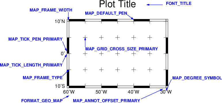
Some GMT parameters that affect plot appearance.
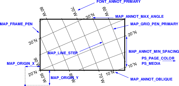
More GMT parameters that affect plot appearance.
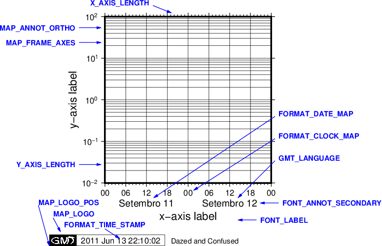
Even more GMT parameters that affect plot appearance.
There are at least two good reasons why the GMT default options are placed in a separate parameter file:
- It would not be practical to allow for command-line syntax covering so many options, many of which are rarely or never changed (such as the ellipsoid used for map projections).
- It is convenient to keep separate
gmt.conffiles for specific projects, so that one may achieve a special effect simply by running GMT commands in the directory whosegmt.conffile has the desired settings. For example, when making final illustrations for a journal article one must often standardize on font sizes and font types, etc. Keeping all those settings in a separategmt.conffile simplifies this process and will allow you to generate those illustrations with the same settings later on. Likewise, GMT scripts that make figures for PowerPoint presentations often use a different color scheme and font size than output intended for laser printers. Organizing these various scenarios into separategmt.conffiles will minimize headaches associated with micro-editing of illustrations.
12.2.2. Changing GMT defaults
As mentioned, GMT programs will attempt to open a file named gmt.conf. At
times it may be desirable to override that default. There are several
ways in which this can be accomplished.
One method is to start each script by saving a copy of the current
gmt.conf, then copying the desiredgmt.conffile to the current directory, and finally reverting the changes at the end of the script. Possible side effects include premature ending of the script due to user error or bugs which means the final resetting does not take place (unless you write your script very carefully.)To permanently change some of the GMT parameters on the fly inside a script the gmtset utility can be used. E.g., to change the primary annotation font to 12 point Times-Bold in red we run
gmt set FONT_ANNOT_PRIMARY 12p,Times-Bold,redThese changes will remain in effect until they are overridden.
If all you want to achieve is to change a few parameters during the execution of a single command but otherwise leave the environment intact, consider passing the parameter changes on the command line via the --PAR=value mechanism. For instance, to temporarily set the output format for floating points to have lots of decimals, say, for map projection coordinate output, append --FORMAT_FLOAT_OUT=%.16lg to the command in question.
Finally, GMT provides to possibility to override the settings only during the running of a single script, reverting to the original settings after the script is run, as if the script was run in “isolation”. The isolation mode is discussed in Section Running GMT in isolation mode.
In addition to those parameters that directly affect the plot there are numerous parameters than modify units, scales, etc. For a complete listing, see the gmt.conf man pages. We suggest that you go through all the available parameters at least once so that you know what is available to change via one of the described mechanisms. The gmt.conf file can be cleared by running gmt clear conf.
12.3. Command line arguments
Each program requires certain arguments specific to its operation. These are explained in the manual pages and in the usage messages. We have tried to choose letters of the alphabet which stand for the argument so that they will be easy to remember. Each argument specification begins with a hyphen (except input file names; see below), followed by a letter, and sometimes a number or character string immediately after the letter. Do not space between the hyphen, letter, and number or string. Do space between options. Example:
gmt pscoast -R0/20/0/20 -Ggray -JM6i -Wthin -B5 -V -P > map.ps
12.4. Standardized command line options
Most of the programs take many of the same arguments such as those related to setting the data region, the map projection, etc. The 26 switches in Table switches have the same meaning in all the programs (although some programs may not use all of them). These options will be described here as well as in the manual pages, as is vital that you understand how to use these options. We will present these options in order of importance (some are used a lot more than others).
| -B | Define tick marks, annotations, and labels for basemaps and axes |
| -J | Select a map projection or coordinate transformation |
| -K | Allow more plot code to be appended to this plot later |
| -O | Allow this plot code to be appended to an existing plot |
| -P | Select Portrait plot orientation [Default is landscape] |
| -R | Define the extent of the map/plot region |
| -U | Plot a time-stamp, by default in the lower left corner of page |
| -V | Select verbose operation; reporting on progress |
| -X | Set the x-coordinate for the plot origin on the page |
| -Y | Set the y-coordinate for the plot origin on the page |
| -a | Associate aspatial data from OGR/GMT files with data columns |
| -b | Select binary input and/or output |
| -d | Replace user nodata values with IEEE NaNs |
| -e | Only process data records that match a pattern |
| -f | Specify the data format on a per column basis |
| -g | Identify data gaps based on supplied criteria |
| -h | Specify that input/output tables have header record(s) |
| -i | Specify which input columns to read |
| -n | Specify grid interpolation settings |
| -o | Specify which output columns to write |
| -p | Control perspective views for plots |
| -r | Set the grid registration to pixel [Default is gridline] |
| -s | Control output of records containing one or more NaNs |
| -t | Change layer PDF transparency |
| -x | Set number of cores to be used in multi-threaded applications |
| -: | Assume input geographic data are (lat,lon) and not (lon,lat) |
12.4.1. Data domain or map region: The -R option
The -R option defines the map region or data domain of interest. It may be specified in one of four ways, two of which are shown in Figure Map region:
- -Rxmin/xmax/ymin/ymax. This is the standard way to specify Cartesian data domains and geographical regions when using map projections where meridians and parallels are rectilinear.
- -Rxlleft/ylleft/xuright/yuright+r. This form is used with map projections that are oblique, making meridians and parallels poor choices for map boundaries. Here, we instead specify the lower left corner and upper right corner geographic coordinates, followed by the modifier +r. This form guarantees a rectangular map even though lines of equal longitude and latitude are not straight lines.
- -Rgridfile. This will copy the domain settings found for the grid in specified file. Note that depending on the nature of the calling program, this mechanism will also set grid spacing and possibly the grid registration (see Section Grid registration: The -r option).
- -Rcodex0/y0/nx/ny. This method can be used when creating grids. Here, code is a 2-character combination of L, C, R (for left, center, or right) and T, M, B for top, middle, or bottom. e.g., BL for lower left. This indicates which point on a rectangular grid region the x0/y0 coordinates refer to, and the grid dimensions nx and ny are used with grid spacings given via -I to create the corresponding region.
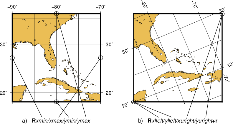
The plot region can be specified in two different ways. (a) Extreme values for each dimension, or (b) coordinates of lower left and upper right corners.
For rectilinear projections the first two forms give identical results. Depending on the selected map projection (or the kind of expected input data), the boundary coordinates may take on several different formats:
- Geographic coordinates:
These are longitudes and latitudes and may be given in decimal degrees (e.g., -123.45417) or in the [±]ddd[:mm[:ss[.xxx]]][W|E|S|N] format (e.g., 123:27:15W). Note that -Rg and -Rd are shorthands for “global domain” -R0/360/-90/90 and -R-180/180/-90/90, respectively.
When used in conjunction with the Cartesian Linear Transformation (-Jx or -JX) —which can be used to map floating point data, geographical coordinates, as well as time coordinates— it is prudent to indicate that you are using geographical coordinates in one of the following ways:
- Use -Rg or -Rd to indicate the global domain.
- Use -Rgxmin/xmax/ymin/ymax to indicate a limited geographic domain.
- Add W, E, S, or N to the coordinate limits or add the generic D or G. Example: -R0/360G/-90/90N.
Alternatively, you may indicate geographical coordinates by supplying -fg; see Section Data type selection: The -f option.
- Projected coordinates:
- These are Cartesian projected coordinates compatible with the chosen projection and are given in a length unit set via the +u modifier, (e.g., -200/200/-300/300+uk for a 400 by 600 km rectangular area centered on the projection center (0, 0). These coordinates are internally converted to the corresponding geographic (longitude, latitude) coordinates for the lower left and upper right corners. This form is convenient when you want to specify a region directly in the projected units (e.g., UTM meters). For allowable units, see Table distunits.
- Calendar time coordinates:
These are absolute time coordinates referring to a Gregorian or ISO calendar. The general format is [date]T[clock], where date must be in the yyyy[-mm[-dd]] (year, month, day-of-month) or yyyy[-jjj] (year and day-of-year) for Gregorian calendars and yyyy[-Www[-d]] (year, week, and day-of-week) for the ISO calendar. If no date is given we assume the current day. The T flag is required if a clock is given.
The optional clock string is a 24-hour clock in hh[:mm[:ss[.xxx]]] format. If no clock is given it implies 00:00:00, i.e., the start of the specified day. Note that not all of the specified entities need be present in the data. All calendar date-clock strings are internally represented as double precision seconds since proleptic Gregorian date Monday January 1 00:00:00 0001. Proleptic means we assume that the modern calendar can be extrapolated forward and backward; a year zero is used, and Gregory’s reforms [11] are extrapolated backward. Note that this is not historical.
- Relative time coordinates:
- These are coordinates which count seconds, hours, days or years relative to a given epoch. A combination of the parameters TIME_EPOCH and TIME_UNIT define the epoch and time unit. The parameter TIME_SYSTEM provides a few shorthands for common combinations of epoch and unit, like j2000 for days since noon of 1 Jan 2000. The default relative time coordinate is that of UNIX computers: seconds since 1 Jan 1970. Denote relative time coordinates by appending the optional lower case t after the value. When it is otherwise apparent that the coordinate is relative time (for example by using the -f switch), the t can be omitted.
- Other coordinates:
- These are simply any coordinates that are not related to geographic or calendar time or relative time and are expected to be simple floating point values such as [±]xxx.xxx[E|e|D|d[±]xx], i.e., regular or exponential notations, with the enhancement to understand FORTRAN double precision output which may use D instead of E for exponents. These values are simply converted as they are to internal representation. [12]
12.4.2. Coordinate transformations and map projections: The -J option
This option selects the coordinate transformation or map projection. The general format is
- -J\(\delta\)[parameters/]scale. Here, \(\delta\) is a lower-case letter of the alphabet that selects a particular map projection, the parameters is zero or more slash-delimited projection parameter, and scale is map scale given in distance units per degree or as 1:xxxxx.
- -J\(\Delta\)[parameters/]width. Here, \(\Delta\) is an upper-case letter of the alphabet that selects a particular map projection, the parameters is zero or more slash-delimited projection parameter, and width is map width (map height is automatically computed from the implied map scale and region).
Since GMT version 4.3.0, there is an alternative way to specify the projections: use the same abbreviation as in the mapping package Proj4. The options thus either look like:
- -Jabbrev/[parameters/]scale. Here, abbrev is a lower-case abbreviation that selects a particular map projection, the parameters is zero or more slash-delimited projection parameter, and scale is map scale given in distance units per degree or as 1:xxxxx.
- -JAbbrev/[parameters/]width. Here, Abbrev is an capitalized abbreviation that selects a particular map projection, the parameters is zero or more slash-delimited projection parameter, and width is map width (map height is automatically computed from the implied map scale and region).
The projections available in GMT are presented in Figure The over-30 map projections and coordinate transformations available in GMT. For details on all GMT projections and the required parameters, see the psbasemap man page. We will also show examples of every projection in the next Chapters, and a quick summary of projection syntax was given in Chapter GMT Overview and Quick Reference.
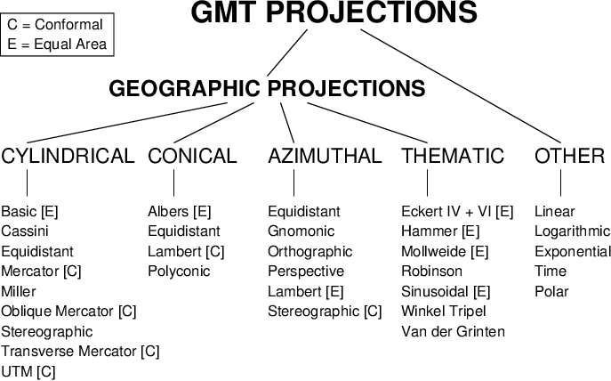
The over-30 map projections and coordinate transformations available in GMT
12.4.3. Map frame and axes annotations: The -B option
This is potentially the most complicated option in GMT, but most examples of its usage are actually quite simple. We distinguish between to sets of information: Frame settings and Axes parameters. These are set separately by their own -B invocations; hence multiple -B specifications may be specified. The frame settings covers things such as which axes should be plotted, canvas fill, plot title, and what type of gridlines be drawn, whereas the Axes settings deal with annotation, tick, and gridline intervals, axes labels, and annotation units.
The Frame settings are specified by
- -B[axes][+b][+gfill][+n][+olon/lat][+ttitle]
Here, the optional axes dictates which of the axes should be drawn and possibly annotated. By default, all 4 map boundaries (or plot axes) are plotted (denoted W, E, S, N). To change this selection, append the codes for those you want (e.g., WSn). In this example, the lower case n denotes to draw the axis and (major and minor) tick marks on the “northern” (top) edge of the plot. The upper case WS will annotate the “western” and “southern” axes with numerals and plot the any axis labels in addition to draw axis/tick-marks. For 3-D plots you can also specify Z or z. By default a single vertical axes will then be plotted at the most suitable map corner. You can override this by appending any combination of corner ids 1234, where 1 represents the lower left corner and the order goes counter-clockwise. Append +b to draw the outline of the 3-D box defined by -R; this modifier is also needed to display gridlines in the x--z, y--z planes. You may paint the map canvas by appending the +gfill modifier [Default is no fill]. If gridlines are specified via the Axes parameters (discussed below) then by default these are referenced to the North pole. If, however, you wish to produce oblique gridlines about another pole you can append +olon/lat to change this behavior (the modifier is ignored if no gridlines are requested). Append +n to have no frame and annotations at all [Default is controlled by the codes]. Finally, you may optionally add +ttitle to place a title that will appear centered above the plot frame.
The Axes settings are specified by
- -B[p|s][x|x|z]intervals[+llabel][+pprefix][+uunit]
but you may also split this into two separate invocations for clarity, i.e.,
- -B[p|s][x|y|z][+llabel][+pprefix][+uunit]
- -B[p|s][x|y|z]intervals
The first optional flag following -B selects p (rimary) [Default] or s (econdary) axes information (which is mostly used for time axes annotations; see examples below). The next optional flags specifies which axes you are providing information for. This can be an individual axis (e.g., just x) or a combination (e.g., xz). If none are given then we default to xy. Thus, if you wish to give different annotation intervals or labels for the various axes then you must repeat the B option for each axis. To add a label to an axis, just append +llabel. If the axis annotation should have a leading text prefix (e.g., dollar sign for those plots of your net worth) you can append +pprefix. For geographic maps the addition of degree symbols, etc. is automatic (and controlled by the GMT default setting FORMAT_GEO_MAP). However, for other plots you can add specific units by adding +uunit. If any of these text strings contain spaces or special UNIX characters you will need to enclose them in quotes. The intervals specification is a concatenated string made up of substrings of the form
[t]stride[phase][u].
The t flag sets the axis item of interest; the available items are listed in Table inttype. Normally, equidistant annotations occur at multiples of stride; you can phase-shift this by appending phase, which can be a positive or negative number.
| Flag | Description |
|---|---|
| a | Annotation and major tick spacing |
| f | Minor tick spacing |
| g | Grid line spacing |
Note that the appearance of certain time annotations (month-, week-, and day-names) may be affected by the GMT_LANGUAGE, FORMAT_TIME_PRIMARY_MAP, and FORMAT_TIME_SECONDARY_MAP settings.
For automated plots the region may not always be the same and thus it can be difficult to determine the appropriate stride in advance. Here GMT provides the opportunity to auto-select the spacing between the major and minor ticks and the grid lines, by not specifying the stride value. For example, -Bafg will select all three spacings automatically for both axes. In case of longitude--latitude plots, this will keep the spacing the same on both axes. You can also use -Bafg/afg to auto-select them separately.
In the case of automatic spacing, when the stride argument is omitted after g, the grid line spacing is chosen the same as the minor tick spacing; unless g is used in consort with a, then the grid lines are spaced the same as the annotations.
The unit flag u can take on one of 18 codes; these are listed in Table units. Almost all of these units are time-axis specific. However, the m and s units will be interpreted as arc minutes and arc seconds, respectively, when a map projection is in effect.
| Flag | Unit | Description |
|---|---|---|
| Y | year | Plot using all 4 digits |
| y | year | Plot using last 2 digits |
| O | month | Format annotation using FORMAT_DATE_MAP |
| o | month | Plot as 2-digit integer (1--12) |
| U | ISO week | Format annotation using FORMAT_DATE_MAP |
| u | ISO week | Plot as 2-digit integer (1--53) |
| r | Gregorian week | 7-day stride from start of week (see TIME_WEEK_START) |
| K | ISO weekday | Plot name of weekday in selected language |
| k | weekday | Plot number of day in the week (1--7) (see TIME_WEEK_START) |
| D | date | Format annotation using FORMAT_DATE_MAP |
| d | day | Plot day of month (1--31) or day of year (1--366) |
| (see FORMAT_DATE_MAP | ||
| R | day | Same as d; annotations aligned with week (see TIME_WEEK_START) |
| H | hour | Format annotation using FORMAT_CLOCK_MAP |
| h | hour | Plot as 2-digit integer (0--24) |
| M | minute | Format annotation using FORMAT_CLOCK_MAP |
| m | minute | Plot as 2-digit integer (0--60) |
| S | seconds | Format annotation using FORMAT_CLOCK_MAP |
| s | seconds | Plot as 2-digit integer (0--60) |
As mentioned, there may be two levels of annotations. Here, “primary” refers to the annotation that is closest to the axis (this is the primary annotation), while “secondary” refers to the secondary annotation that is plotted further from the axis. The examples below will clarify what is meant. Note that the terms “primary” and “secondary” do not reflect any hierarchical order of units: The “primary” annotation interval is usually smaller (e.g., days) while the “secondary” annotation interval typically is larger (e.g., months).
12.4.3.1. Geographic basemaps
Geographic basemaps may differ from regular plot axis in that some projections support a “fancy” form of axis and is selected by the MAP_FRAME_TYPE setting. The annotations will be formatted according to the FORMAT_GEO_MAP template and MAP_DEGREE_SYMBOL setting. A simple example of part of a basemap is shown in Figure Geographic map border.
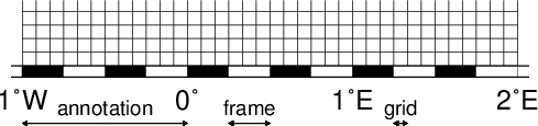
Geographic map border using separate selections for annotation, frame, and grid intervals. Formatting of the annotation is controlled by the parameter FORMAT_GEO_MAP in your gmt.conf.
The machinery for primary and secondary annotations introduced for time-series axes can also be utilized for geographic basemaps. This may be used to separate degree annotations from minutes- and seconds-annotations. For a more complicated basemap example using several sets of intervals, including different intervals and pen attributes for grid lines and grid crosses, see Figure Complex basemap.
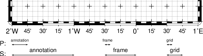
Geographic map border with both primary (P) and secondary (S) components.
12.4.3.2. Cartesian linear axes
For non-geographic axes, the MAP_FRAME_TYPE setting is implicitly set to plain. Other than that, cartesian linear axes are very similar to geographic axes. The annotation format may be controlled with the FORMAT_FLOAT_OUT parameter. By default, it is set to “%g”, which is a C language format statement for floating point numbers [13], and with this setting the various axis routines will automatically determine how many decimal points should be used by inspecting the stride settings. If FORMAT_FLOAT_OUT is set to another format it will be used directly (.e.g, “%.2f” for a fixed, two decimals format). Note that for these axes you may use the unit setting to add a unit string to each annotation (see Figure Axis label).
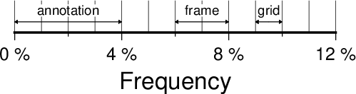
Linear Cartesian projection axis. Long tick-marks accompany
annotations, shorter ticks indicate frame interval. The axis label is
optional. For this example we used -R0/12/0/0.95 -JX3i/0.3i -Ba4f2g1+lFrequency+u" %" -BS
12.4.3.3. Cartesian log10 axes
Due to the logarithmic nature of annotation spacings, the stride parameter takes on specific meanings. The following concerns are specific to log axes (see Figure Logarithmic projection axis):
- stride must be 1, 2, 3, or a negative integer -n. Annotations/ticks will then occur at 1, 1-2-5, or 1,2,3,4,…,9, respectively, for each magnitude range. For -n the annotations will take place every n’th magnitude.
- Append l to stride. Then, log10 of the annotation is plotted at every integer log10 value (e.g., x = 100 will be annotated as “2”) [Default annotates x as is].
- Append p to stride. Then, annotations appear as 10 raised to log10 of the value (e.g., 10-5).
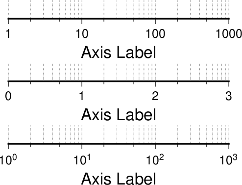
Logarithmic projection axis using separate values for annotation, frame, and grid intervals. (top) Here, we have chosen to annotate the actual values. Interval = 1 means every whole power of 10, 2 means 1, 2, 5 times powers of 10, and 3 means every 0.1 times powers of 10. We used -R1/1000/0/1 -JX3il/0.25i -Ba1f2g3. (middle) Here, we have chosen to annotate \(\log_{10}\) of the actual values, with -Ba1f2g3l. (bottom) We annotate every power of 10 using \(\log_{10}\) of the actual values as exponents, with -Ba1f2g3p.
12.4.3.4. Cartesian exponential axes
Normally, stride will be used to create equidistant (in the user’s unit) annotations or ticks, but because of the exponential nature of the axis, such annotations may converge on each other at one end of the axis. To avoid this problem, you can append p to stride, and the annotation interval is expected to be in transformed units, yet the annotation itself will be plotted as un-transformed units (see Figure Power projection axis). E.g., if stride = 1 and power = 0.5 (i.e., sqrt), then equidistant annotations labeled 1, 4, 9, … will appear.
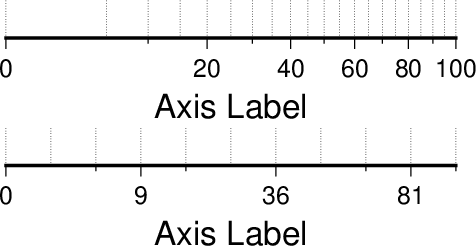
Exponential or power projection axis. (top) Using an exponent of 0.5 yields a \(sqrt(x)\) axis. Here, intervals refer to actual data values, in -R0/100/0/0.9 -JX3ip0.5/0.25i -Ba20f10g5. (bottom) Here, intervals refer to projected values, although the annotation uses the corresponding unprojected values, as in -Ba3f2g1p.
12.4.3.5. Cartesian time axes
What sets time axis apart from the other kinds of plot axes is the numerous ways in which we may want to tick and annotate the axis. Not only do we have both primary and secondary annotation items but we also have interval annotations versus tick-mark annotations, numerous time units, and several ways in which to modify the plot. We will demonstrate this flexibility with a series of examples. While all our examples will only show a single x-axis (south, selected via -BS), time-axis annotations are supported for all axes.
Our first example shows a time period of almost two months in Spring 2000. We want to annotate the month intervals as well as the date at the start of each week:
gmt set FORMAT_DATE_MAP=-o FONT_ANNOT_PRIMARY +9p
gmt psbasemap -R2000-4-1T/2000-5-25T/0/1 -JX5i/0.2i -Bpa7Rf1d -Bsa1O -BS -P > GMT_-B_time1.ps
These commands result in Figure Cartesian time axis. Note the leading hyphen in the FORMAT_DATE_MAP removes leading zeros from calendar items (e.g., 02 becomes 2).

Cartesian time axis, example 1
The next example shows two different ways to annotate an axis portraying 2 days in July 1969:
gmt set FORMAT_DATE_MAP "o dd" FORMAT_CLOCK_MAP hh:mm FONT_ANNOT_PRIMARY +9p
gmt psbasemap -R1969-7-21T/1969-7-23T/0/1 -JX5i/0.2i -Bpa6Hf1h -Bsa1K -BS -P -K > GMT_-B_time2.ps
gmt psbasemap -R -J -Bpa6Hf1h -Bsa1D -BS -O -Y0.65i >> GMT_-B_time2.ps
The lower example (Figure Cartesian time axis, example 2) chooses to annotate the weekdays (by specifying a1K) while the upper example choses dates (by specifying a1D). Note how the clock format only selects hours and minutes (no seconds) and the date format selects a month name, followed by one space and a two-digit day-of-month number.
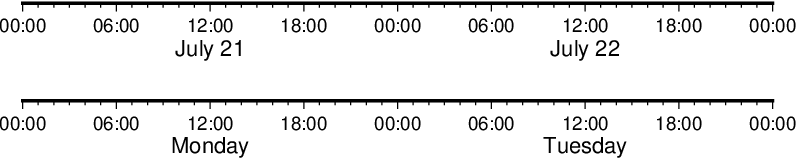
Cartesian time axis, example 2
The third example (Figure Cartesian time axis, example 3) presents two years, annotating both the years and every 3rd month.
gmt set FORMAT_DATE_MAP o FORMAT_TIME_PRIMARY_MAP Character FONT_ANNOT_PRIMARY +9p
gmt psbasemap -R1997T/1999T/0/1 -JX5i/0.2i -Bpa3Of1o -Bsa1Y -BS -P > GMT_-B_time3.ps
Note that while the year annotation is centered on the 1-year interval, the month annotations must be centered on the corresponding month and not the 3-month interval. The FORMAT_DATE_MAP selects month name only and FORMAT_TIME_PRIMARY_MAP selects the 1-character, upper case abbreviation of month names using the current language (selected by GMT_LANGUAGE).

Cartesian time axis, example 3
The fourth example (Figure Cartesian time axis, example 4) only shows a few hours of a day, using relative time by specifying t in the -R option while the TIME_UNIT is d (for days). We select both primary and secondary annotations, ask for a 12-hour clock, and let time go from right to left:
gmt set FORMAT_CLOCK_MAP=-hham FONT_ANNOT_PRIMARY +9p TIME_UNIT d
gmt psbasemap -R0.2t/0.35t/0/1 -JX-5i/0.2i -Bpa15mf5m -Bsa1H -BS -P > GMT_-B_time4.ps

Cartesian time axis, example 4
The fifth example shows a few weeks of time (Figure Cartesian time axis, example 5). The lower axis shows ISO weeks with week numbers and abbreviated names of the weekdays. The upper uses Gregorian weeks (which start at the day chosen by TIME_WEEK_START); they do not have numbers.
gmt set FORMAT_DATE_MAP u FORMAT_TIME_PRIMARY_MAP Character \
       FORMAT_TIME_SECONDARY_MAP full FONT_ANNOT_PRIMARY +9p
gmt psbasemap -R1969-7-21T/1969-8-9T/0/1 -JX5i/0.2i -Bpa1K -Bsa1U -BS -P -K > GMT_-B_time5.ps
gmt set FORMAT_DATE_MAP o TIME_WEEK_START Sunday FORMAT_TIME_SECONDARY_MAP Chararacter
gmt psbasemap -R -J -Bpa3Kf1k -Bsa1r -BS -O -Y0.65i >> GMT_-B_time5.ps
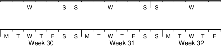
Cartesian time axis, example 5
Our sixth example (Figure Cartesian time axis, example 6) shows the first five months of 1996, and we have annotated each month with an abbreviated, upper case name and 2-digit year. Only the primary axes information is specified.
gmt set FORMAT_DATE_MAP "o yy" FORMAT_TIME_PRIMARY_MAP Abbreviated
gmt psbasemap -R1996T/1996-6T/0/1 -JX5i/0.2i -Ba1Of1d -BS -P > GMT_-B_time6.ps

Cartesian time axis, example 6
Our seventh and final example (Figure Cartesian time axis, example 7) illustrates annotation of year-days. Unless we specify the formatting with a leading hyphen in FORMAT_DATE_MAP we get 3-digit integer days. Note that in order to have the two years annotated we need to allow for the annotation of small fractional intervals; normally such truncated interval must be at least half of a full interval.
gmt set FORMAT_DATE_MAP jjj TIME_INTERVAL_FRACTION 0.05 FONT_ANNOT_PRIMARY +9p
gmt psbasemap -R2000-12-15T/2001-1-15T/0/1 -JX5i/0.2i -Bpa5Df1d -Bsa1Y -BS -P > GMT_-B_time7.ps

Cartesian time axis, example 7
12.4.3.6. Custom axes
Irregularly spaced annotations or annotations based on look-up tables can be implemented using the custom annotation mechanism. Here, we given the c (custom) type to the -B option followed by a filename that contains the annotations (and tick/grid-lines specifications) for one axis. The file can contain any number of comments (lines starting with #) and any number of records of the format
The coord is the location of the desired annotation, tick, or grid-line, whereas type is a string composed of letters from a (annotation), i interval annotation, f frame tick, and g gridline. You must use either a or i within one file; no mixing is allowed. The coordinates should be arranged in increasing order. If label is given it replaces the normal annotation based on the coord value. Our last example (Figure Custom and irregular annotations) shows such a custom basemap with an interval annotations on the x-axis and irregular annotations on the y-axis.
cat << EOF > xannots.txt
416.0 ig Devonian
443.7 ig Silurian
488.3 ig Ordovician
542 ig Cambrian
EOF
cat << EOF > yannots.txt
0 a
1 a
2 f
2.71828 ag e
3 f
3.1415926 ag @~p@~
4 f
5 f
6 f
6.2831852 ag 2@~p@~
EOF
gmt psbasemap -R416/542/0/6.2831852 -JX-5i/2.5i -Bpx25f5g25+u" Ma" -Bpycyannots.txt \
              -BWS+glightblue -P -K > GMT_-B_custom.ps
gmt psbasemap -R416/542/0/6.2831852 -JX-5i/2.5i -Bsxcxannots.txt -BWS -O \
              --MAP_ANNOT_OFFSET_SECONDARY=10p --MAP_GRID_PEN_SECONDARY=2p >> GMT_-B_custom.ps
rm -f [xy]annots.txt
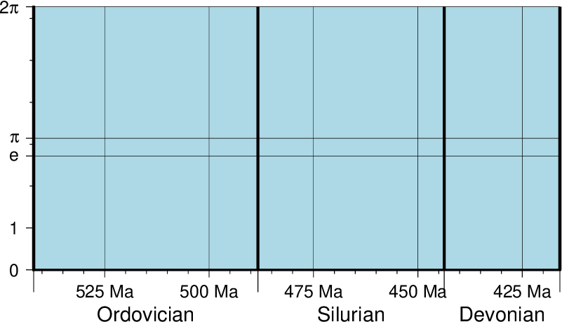
Custom and irregular annotations, tick-marks, and gridlines.
12.4.4. Portrait plot orientation: The -P option
The -P option selects Portrait plotting mode [14]. In general, a plot has an x-axis increasing from left to right and a y-axis increasing from bottom to top. If the paper is turned so that the long dimension of the paper is parallel to the x-axis then the plot is said to have Landscape orientation. If the long dimension of the paper parallels the y-axis the orientation is called Portrait (think of taking pictures with a camera and these words make sense). The default Landscape orientation is obtained by translating the origin in the x-direction (by the width of the chosen paper PS_MEDIA) and then rotating the coordinate system counterclockwise by 90. By default the PS_MEDIA is set to Letter (or A4 if SI is chosen); this value must be changed when using different media, such as 11” x 17” or large format plotters (Figure Plot orientation).

Users can specify Landscape [Default] or Portrait -P) orientation.
12.4.5. Plot overlays: The -K -O options
The -K and -O options control the generation of PostScript code for multiple overlay plots. All PostScript files must have a header (for initializations), a body (drawing the figure), and a trailer (printing it out) (see Figure Multiple overlay plots). Thus, when overlaying several GMT plots we must make sure that the first plot call omits the trailer, that all intermediate calls omit both header and trailer, and that the final overlay omits the header. The -K omits the trailer which implies that more PostScript code will be appended later [Default terminates the plot system]. The -O selects Overlay plot mode and omits the header information [Default initializes a new plot system]. Most unexpected results for multiple overlay plots can be traced to the incorrect use of these options. If you run only one plot program, ignore both the -O and -K options; they are only used when stacking plots.
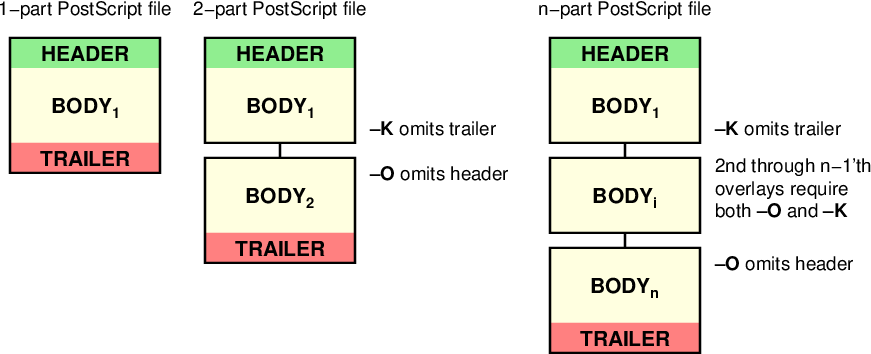
A final PostScript file consists of any number of individual pieces.
12.4.6. Timestamps on plots: The -U option
The -U option draws UNIX System time stamp. Optionally, append an arbitrary text string (surrounded by double quotes), or the code c, which will plot the current command string (Figure Time stamp).

The -U option makes it easy to date a plot.
12.4.7. Verbose feedback: The -V option
The -V option selects verbose mode, which will send progress reports to standard error. Even more verbose levels are -Vl (long verbose) and -Vd (debug). Normal verbosity level produces only error and warning messages. This is the default or can be selected by using -Vn. If compiled with backward-compatibility support, the default is -Vc, which includes warnings about deprecated usage. Finally, -Vq can be used to run without any warnings or errors. This option can also be set by specifying the default GMT_VERBOSE, as quiet, normal, compat, verbose, long_verbose, or debug, in order of increased verbosity.
12.4.8. Plot positioning and layout: The -X -Y options
The -X and -Y options shift origin of plot by (xoff,yoff) inches (Default is (MAP_ORIGIN_X, MAP_ORIGIN_Y) for new plots [15] and (0,0) for overlays (-O)). By default, all translations are relative to the previous origin (see Figure Plot positioning). Supply offset as c to center the plot in that direction relative to the page margin. Absolute translations (i.e., relative to a fixed point (0,0) at the lower left corner of the paper) can be achieve by prepending “a” to the offsets. Subsequent overlays will be co-registered with the previous plot unless the origin is shifted using these options. The offsets are measured in the current coordinates system (which can be rotated using the initial -P option; subsequent -P options for overlays are ignored).
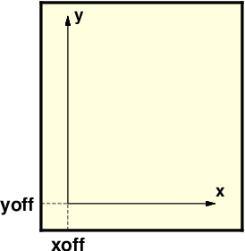
Plot origin can be translated freely with -X -Y.
12.4.9. OGR/GMT GIS i/o: The -a option
GMT relies on external tools to translate geospatial files such as shapefiles into a format we can read. The tool ogr2ogr in the GDAL package can do such translations and preserve the aspatial metadata via a new OGR/GMT format specification (See Chapter The GMT Vector Data Format for OGR Compatibility). For this to be useful we need a mechanism to associate certain metadata values with required input and output columns expected by GMT programs. The -a option allows you to supply one or more comma-separated associations col=name, where name is the name of an aspatial attribute field in a OGR/GMT file and whose value we wish to as data input for column col. The given aspatial field thus replaces any other value already set. Note that col = 0 is the first data columns. Note that if no aspatial attributes are needed then the -a option is not needed -- GMT will still process and read such data files.
12.4.9.1. OGR/GMT input with -a option
If you need to populate GMT data columns with (constant) values specified by aspatial attributes, use -a and append any number of comma-separated col=name associations. E.g., 2=depth will read the spatial x,y columns from the file and add a third (z) column based on the value of the aspatial field called depth. You can also associate aspatial fields with other settings such as labels, fill colors, pens, and values used to look-up colors. Do so by letting the col value be one of D, G, L, T, W, or Z. This works analogously to how standard multi-segment files can pass such options via its segment headers (See Chapter GMT file formats).
12.4.9.2. OGR/GMT output with -a option
You can also make GMT table-writing tools output the OGR/GMT format directly. Again, specify if certain GMT data columns with constant values should be stored as aspatial metadata using the col=name[:type], where you can optionally specify what data type it should be (double, integer, string, logical, byte, or datetime) [double is default]. As for input, you can also use the special col entries of D, G, L, T, W, or Z to have values stored as options in segment headers be used as the source for the name aspatial field. Finally, for output you must append +ggeometry, where geometry can be any of [M]POINT|LINE|POLY; the M represent the multi-versions of these three geometries. Use upper-case +G to signal that you want to split any line or polygon features that straddle the Dateline.
12.4.10. Binary table i/o: The -b option
All GMT programs that accept table data input may read ASCII, native binary, or netCDF tables. Native binary files may have a header section and the -hn option (see Section Header data records: The -h option) can be used to skip the first n bytes. The data record can be in any format, you may mix different data types and even byte-swap individual columns or the entire record. When using native binary data the user must be aware of the fact that GMT has no way of determining the actual number of columns in the file. You must therefore pass that information to GMT via the binary -bi nt option, where n is the number of data columns of given type t, where t must be one of c (signed 1-byte character, int8_t), u (unsigned 1-byte character, uint8_t), h (signed 2-byte int, int16_t), H (unsigned 2-byte int, uint16_t), i (signed 4-byte int, int32_t), I (unsigned 4-byte int, uint32_t), l (signed 8-byte int, int64_t), L (unsigned 8-byte int, uint64_t), f (4-byte single-precision float), and d (8-byte double-precision float). In addition, use x to skip n bytes anywhere in the record. For a mixed-type data record you can concatenate several [n]t combinations, separated by commas. You may append w to any of the items to force byte-swapping. Alternatively, append +L|B to indicate that the entire data file should be read or written as little- or big-endian, respectively. Here, n is the number of each item in your binary file. Note that n may be larger than m, the number of columns that the GMT program requires to do its task. If n is not given then it defaults to m and all columns are assumed to be of the single specified type t [d (double), if not set]. If n < m an error is generated. Multiple segment files are allowed and the segment headers are assumed to be records where all the fields equal NaN.
For native binary output, use the -bo option; see -bi for further details.
Because of its meta data, reading netCDF tables (i.e., netCDF files containing 1-dimensional arrays) is quite a bit less complex than reading native binary files. When feeding netCDF tables to programs like psxy, the program will automatically recognize the format and read whatever amount of columns are needed for that program. To steer which columns are to be read, the user can append the suffix ?var1/var2/… to the netCDF file name, where var1, var2, etc. are the names of the variables to be processed. No -bi option is needed in this case.
Currently, netCDF tables can only be input, not output. For more information, see Chapter GMT file formats.
12.4.11. Missing data conversion: The -d option
Within GMT, any missing values are represented by the IEEE NaN value. However, there are occasionally the need to handle user data where missing data are represented by some unlikely data value such as -99999. Since GMT cannot guess that in your data set -99999 is a special value, you can use the -d option to have such values replaced with NaNs. Similarly, should your GMT output need to conform to such a requirement you can replace all NaNs with the chosen nodata value. If only input or output should be affected, use -di or -do, respectably.
12.4.12. Data record pattern matching: The -e option
Modules that read ASCII tables will normally process all the data records that are read. The -e option offers a built in pattern scanner that will only pass records that match the given patterns or regular expressions. The test can also be inverted to only pass data records that do not match the pattern. The test does not apply to header or segment headers.
12.4.13. Data type selection: The -f option
When map projections are not required we must explicitly state what kind of data each input or output column contains. This is accomplished with the -f option. Following an optional i (for input only) or o (for output only), we append a text string with information about each column (or range of columns) separated by commas. Each string starts with the column number (0 is first column) followed by either x (longitude), y (latitude), T (absolute calendar time) or t (relative time). If several consecutive columns have the same format you may specify a range of columns rather than a single column, i.e., 0--4 for the first 5 columns. For example, if our input file has geographic coordinates (latitude, longitude) with absolute calendar coordinates in the columns 3 and 4, we would specify fi0y,1x,3--4T. All other columns are assumed to have the default, floating point format and need not be set individually. The shorthand -f[i|o]g means -f[i|o]0x,1y (i.e., geographic coordinates). A special use of -f is to select -fp[unit], which requires -J and lets you use projected map coordinates (e.g., UTM meters) as data input. Such coordinates are automatically inverted to longitude, latitude during the data import. Optionally, append a length unit (see Table distunits) [meter]. For more information, see Sections Input data formats and Output data formats.
12.4.14. Data gap detection: The -g option
GMT has several mechanisms that can determine line segmentation. Typically, data segments are separated by multiple segment header records (see Chapter GMT file formats). However, if key data columns contain a NaN we may also use that information to break lines into multiple segments. This behavior is modified by the parameter IO_NAN_RECORDS which by default is set to skip, meaning such records are considered bad and simply skipped. If you wish such records to indicate a segment boundary then set this parameter to pass. Finally, you may wish to indicate gaps based on the data values themselves. The -g option is used to detect gaps based on one or more criteria (use -g+ if all the criteria must be met; otherwise only one of the specified criteria needs to be met to signify a data gap). Gaps can be based on excessive jumps in the x- or y-coordinates (-gx or -gy), or on the distance between points (-gd). Append the gap distance and optionally a unit for actual distances. For geographic data the optional unit may be arc degree, minute, and second, or meter [Default], feet, kilometer, Miles, or nautical miles. For programs that map data to map coordinates you can optionally specify these criteria to apply to the projected coordinates (by using upper-case -gX, -gY or -gD). In that case, choose from centimeter, inch or point [Default unit is controlled by PROJ_LENGTH_UNIT]. Note: For -gx or -gy with time data the unit is instead controlled by TIME_UNIT.
12.4.15. Header data records: The -h option
The -h[i|o][n_recs] option lets GMT know that input file(s) have n_recs header records [0]. If there are more than one header record you must specify the number after the -h option, e.g., -h4. Note that blank lines and records that start with the character # are automatically considered header records and skipped. Thus, n_recs refers to general text lines that do not start with # and thus must specifically be skipped in order for the programs to function properly. The default number of such header records if -h is used is one of the many parameters in the gmt.conf file (IO_N_HEADER_RECS, by default 0), but can be overridden by -hn_header_recs. Normally, programs that both read and write tables will output the header records that are found on input. Use -hi to suppress the writing of header records. You can use the -h options modifiers to to tell programs to output extra header records for titles, remarks or column names identifying each data column.
When -b is used to indicate binary data the -h takes on a slightly different meaning. Now, the n_recs argument is taken to mean how many bytes should be skipped (on input) or padded with the space character (on output).
12.4.16. Input columns selection: The -i option
The -icolumns option allows you to specify which input file data columns to use and in what order. By default, GMT will read all the data columns in the file, starting with the first column (0). Using -i modifies that process. For instance, to use the 4th, 7th, and 3rd data column as the required x,y,z to blockmean you would specify -i3,6,2 (since 0 is the first column). The chosen data columns will be used as is. Optionally, you can specify that input columns should be transformed according to a linear or logarithmic conversion. Do so by appending [l][sscale][ooffset] to each column (or range of columns). All items are optional: The l implies we should first take \(\log_{10}\) of the data [leave as is]. Next, we may scale the result by the given scale [1]. Finally, we add in the specified offset [0].
12.4.17. Grid interpolation parameters: The -n option
The -ntype option controls parameters used for 2-D grids resampling. You can select the type of spline used (-nb for B-spline smoothing, -nc for bicubic [Default], -nl for bilinear, or -nn for nearest-node value). For programs that support it, antialiasing is by default on; optionally, append +a to switch off antialiasing. By default, boundary conditions are set according to the grid type and extent. Change boundary conditions by appending +bBC, where BC is either g for geographic boundary conditions or one (or both) of n and p for natural or periodic boundary conditions, respectively. Append x or y to only apply the condition in one dimension. E.g., -nb+nxpy would imply natural boundary conditions in the x direction and periodic conditions in the y direction. Finally, append +tthreshold to control how close to nodes with NaN the interpolation should go. A threshold of 1.0 requires all (4 or 16) nodes involved in the interpolation to be non-NaN. 0.5 will interpolate about half way from a non-NaN value; 0.1 will go about 90% of the way, etc.
12.4.18. Output columns selection: The -o option
The -ocolumns option allows you to specify which columns to write on output and in what order. By default, GMT will write all the data columns produced by the program. Using -o modifies that process. For instance, to write just the 4th and 2nd data column to the output you would use -o3,1 (since 0 is the first column). You can also use a column more than once, e.g., -o3,1,3, to duplicate a column on output.
12.4.19. Perspective view: The -p option
All plotting programs that normally produce a flat, two-dimensional illustration can be told to view this flat illustration from a particular vantage point, resulting in a perspective view. You can select perspective view with the -p option by setting the azimuth and elevation of the viewpoint [Default is 180/90]. When -p is used in consort with -Jz or -JZ, a third value can be appended which indicates at which z-level all 2-D material, like the plot frame, is plotted (in perspective) [Default is at the bottom of the z-axis]. For frames used for animation, you may want to append + to fix the center of your data domain (or specify a particular world coordinate point with +wlon0/lat[z]) which will project to the center of your page size (or you may specify the coordinates of the projected view point with +vx0/y0. When -p is used without any further arguments, the values from the last use of -p in a previous GMT command will be used. Alternatively, you can perform a simple rotation about the z-axis by just giving the rotation angle. Optionally, use +v or +w to select another axis location than the plot origin.
12.4.20. Grid registration: The -r option
All 2-D grids in GMT have their nodes organized in one of two ways, known as gridline- and pixel- registration. The GMT default is gridline registration; programs that allow for the creation of grids can use the -r option to select pixel registration instead. Most observed data tend to be in gridline registration while processed data sometime may be distributed in pixel registration. While you may convert between the two registrations this conversion looses the Nyquist frequency and dampens the other high frequencies. It is best to avoid any registration conversion if you can help it. Planning ahead may be important.
12.4.20.1. Gridline registration
In this registration, the nodes are centered on the grid line intersections and the data points represent the average value in a cell of dimensions (\(x_{inc} \cdot y_{inc}\)) centered on each node (left side of Figure Grid registration). In the case of grid line registration the number of nodes are related to region and grid spacing by
which for the example in left side of Figure Gridline registration yields nx = ny = 4.
12.4.20.2. Pixel registration
Here, the nodes are centered in the grid cells, i.e., the areas between grid lines, and the data points represent the average values within each cell (right side of Figure Grid registration). In the case of pixel registration the number of nodes are related to region and grid spacing by
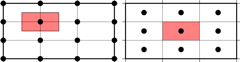
Gridline- and pixel-registration of data nodes.
Thus, given the same region (-R) and grid spacing, the pixel-registered grids have one less column and one less row than the gridline-registered grids; here we find nx = ny = 3.
12.4.21. NaN-record treatment: The -s option
We can use this option to suppress output for records whose z-value equals NaN (by default we output all records). Alternatively, append r to reverse the suppression, i.e., only output the records whose z-value equals NaN. Use -sa to suppress output records where one or more fields (and not necessarily z) equal NaN. Finally, you can supply a comma-separated list of all columns or column ranges to consider for this NaN test.
12.4.22. Layer PDF transparency: The -t option
While the PostScript language does not support transparency, PDF does, and via PostScript extensions one can manipulate the transparency levels of objects. The -t option allows you to change the transparency level for the current overlay by appending a percentage in the 0--100 range; the default is 0, or opaque. Transparency may also be controlled on a feature by feature basis when setting color or fill (see section Specifying area fill attributes).
12.4.23. Latitude/Longitude or Longitude/Latitude?: The -: option
For geographical data, the first column is expected to contain longitudes and the second to contain latitudes. To reverse this expectation you must apply the -: option. Optionally, append i or o to restrict the effect to input or output only. Note that command line arguments that may take geographic coordinates (e.g., -R) always expect longitude before latitude. Also, geographical grids are expected to have the longitude as first (minor) dimension.
12.5. Command line history
GMT programs “remember” the standardized command line options (See Section Standardized command line options) given during their previous invocations and this provides a shorthand notation for complex options. For example, if a basemap was created with an oblique Mercator projection, specified as
-Joc170W/25:30S/33W/56:20N/1:500000
then a subsequent psxy command to plot
symbols only needs to state -Jo in order to activate the same
projection. In contrast, note that -J by itself will pick the most
recently used projection. Previous commands are maintained in the file gmt.history,
of which there will be one in each directory you run the programs from.
This is handy if you create separate directories for separate projects
since chances are that data manipulations and plotting for each project
will share many of the same options. Note that an option spelled out on
the command line will always override the previous entry in the gmt.history file and, if
execution is successful, will replace this entry as the previous option
argument in the gmt.history file. If you call several GMT modules piped together
then GMT cannot guarantee that the gmt.history file is processed in the intended
order from left to right. The only guarantee is that the file will not
be clobbered since GMT uses advisory file locking. The uncertainty in
processing order makes the use of shorthands in pipes unreliable. We
therefore recommend that you only use shorthands in single process
command lines, and spell out the full command option when using chains
of commands connected with pipes. The history can be cleared by running
gmt clear history.
12.6. Usage messages, syntax- and general error messages
Each program carries a usage message. If you enter the program name without any arguments, the program will write the complete usage message to standard error (your screen, unless you redirect it). This message explains in detail what all the valid arguments are. If you enter the program name followed by a hyphen (-) only you will get a shorter version which only shows the command line syntax and no detailed explanations. If you incorrectly specify an option or omit a required option, the program will produce syntax errors and explain what the correct syntax for these options should be. If an error occurs during the running of a program, the program will in some cases recognize this and give you an error message. Usually this will also terminate the run. The error messages generally begin with the name of the program in which the error occurred; if you have several programs piped together this tells you where the trouble is.
12.7. Standard input or file, header records
Most of the programs which expect table data input can read either standard input or input in one or several files. These programs will try to read stdin unless you type the filename(s) on the command line without the above hyphens. (If the program sees a hyphen, it reads the next character as an instruction; if an argument begins without a hyphen, it tries to open this argument as a filename). This feature allows you to connect programs with pipes if you like. If your input is ASCII and has one or more header records that do not begin with #, you must use the -h option (see Section Header data records: The -h option). ASCII files may in many cases also contain segment-headers separating data segments. These are called “multi-segment files”. For binary table data the -h option may specify how many bytes should be skipped before the data section is reached. Binary files may also contain segment-headers separating data segments. These segment-headers are simply data records whose fields are all set to NaN; see Chapter GMT file formats for complete documentation.
If filenames are given for reading, GMT programs will first look for them in the current directory. If the file is not found, the programs will look in other directories pointed to by the directory parameters DIR_DATA, directory parameters DIR_CACHE and or by the environmental parameters $GMT_USERDIR, $GMT_CACHEDIR and $GMT_DATADIR (if set). They may be set by the user to point to directories that contain data sets of general use, thus eliminating the need to specify a full path to these files. Usually, the DIR_DATA directory will hold data sets of a general nature (tables, grids), whereas the $GMT_USERDIR directory (its default value is $HOME/.gmt) may hold miscellaneous data sets more specific to the user; this directory also stores GMT defaults and other configuration files. The DIR_CACHE will typically contain data files downloaded automatically by GMT modules. See directory parameters for details. Program output is always written to the current directory unless a full path has been specified.
12.8. URLs and special files
Three classes of files are given special treatment in GMT.
- Some data sets are ubiquitous and used by nearly all GMT users. At the moment this set is limited to Earth relief grids. If you reference files called earth_relief_res.grd on a command line then that grid will automatically be downloaded from the GMT Data Site and placed in $GMT_USERDIR [~/.gmt]. The resolution res allows a choice among 13 command grid spacings: 60m, 30m, 20m, 15m, 10m, 6m, 5m, 4m, 3m, 2m, 1m, 30s, and 15s (with file sizes 111 kb, 376 kb, 782 kb, 1.3 Mb, 2.8 Mb, 7.5 Mb, 11 Mb, 16 Mb, 27 Mb, 58 Mb, 214 Mb, 778 Mb, and 2.6 Gb respectively). Once one of these have been downloaded any future reference will simply obtain the file from $GMT_USERDIR (except if explicitly removed by the user). Note: The four highest resolutions are the original data sets SRTM15+, SRTM30+, ETOPO1 and ETOPO2V2. Lower resolutions are spherically Gaussian-filtered versions of ETOPO1.
- If a file is given as a full URL, starting with http://, https://, or ftp://, then the file will be downloaded to DIR_CACHE and subsequently read from there (until removed by the user). If the URL is actually a CGI Get command (i.e., ends in ?par=val1&par2=val2…) then we download the file each time we encounter the URL.
- Demonstration files used in online documentation, example scripts, or even the large test suite may be given in the format @filename. When such a file is encountered on the command line it is understood to be a short-hand representation of the full URL to filename on the GMT Cache Data FTP site. Since this address may change over time we use the leading @ to simplify access to these files. Such files will also be downloaded to DIR_CACHE and subsequently read from there (until removed by the user).
The user cache (DIR_CACHE) and all its contents can be cleared any time via the command gmt clear cache.
12.9. Verbose operation
Most of the programs take an optional -V argument which will run the program in the “verbose” mode (see Section Verbose feedback: The -V option). Verbose will write to standard error information about the progress of the operation you are running. Verbose reports things such as counts of points read, names of data files processed, convergence of iterative solutions, and the like. Since these messages are written to stderr, the verbose talk remains separate from your data output. You may optionally choose among five models of verbosity; each mode adds more messages with an increasing level of details. The modes are
q Complete silence, not even fatal error messages.
n Warnings and progress messages [Default].
c Warnings about deprecated usage (if compiled for compatibility).
l Detailed progress messages.
d Debugging messages.
The verbosity is cumulative, i.e., mode l means all messages of mode n as well. will be reported.
12.10. Program output
Most programs write their results, including PostScript plots, to standard output. The exceptions are those which may create binary netCDF grid files such as surface (due to the design of netCDF a filename must be provided; however, alternative binary output formats allowing piping are available; see Section Grid file format specifications). Most operating systems let you can redirect standard output to a file or pipe it into another process. Error messages, usage messages, and verbose comments are written to standard error in all cases. You can usually redirect standard error as well, if you want to create a log file of what you are doing. The syntax for redirection differ among the main shells (Bash and C-shell) and is a bit limited in DOS.
12.11. Input data formats
Most of the time, GMT will know what kind of x and y coordinates it is reading because you have selected a particular coordinate transformation or map projection. However, there may be times when you must explicitly specify what you are providing as input using the -f switch. When binary input data are expected (-bi) you must specify exactly the format of the records. However, for ASCII input there are numerous ways to encode data coordinates (which may be separated by white-space or commas). Valid input data are generally of the same form as the arguments to the -R option (see Section Data domain or map region: The -R option), with additional flexibility for calendar data. Geographical coordinates, for example, can be given in decimal degrees (e.g., -123.45417) or in the [±]ddd[:mm[:ss[.xxx]]][W|E|S|N] format (e.g., 123:27:15W). With -fp you may even supply projected data like UTM coordinates.
Because of the widespread use of incompatible and ambiguous formats, the processing of input date components is guided by the template FORMAT_DATE_IN in your gmt.conf file; it is by default set to yyyy-mm-dd. Y2K-challenged input data such as 29/05/89 can be processed by setting FORMAT_DATE_IN to dd/mm/yy. A complete description of possible formats is given in the gmt.conf man page. The clock string is more standardized but issues like 12- or 24-hour clocks complicate matters as well as the presence or absence of delimiters between fields. Thus, the processing of input clock coordinates is guided by the template FORMAT_CLOCK_IN which defaults to hh:mm:ss.xxx.
GMT programs that require a map projection argument will implicitly know what kind of data to expect, and the input processing is done accordingly. However, some programs that simply report on minimum and maximum values or just do a reformatting of the data will in general not know what to expect, and furthermore there is no way for the programs to know what kind of data other columns (beyond the leading x and y columns) contain. In such instances we must explicitly tell GMT that we are feeding it data in the specific geographic or calendar formats (floating point data are assumed by default). We specify the data type via the -f option (which sets both input and output formats; use -fi and -fo to set input and output separately). For instance, to specify that the the first two columns are longitude and latitude, and that the third column (e.g., z) is absolute calendar time, we add -fi0x,1y,2T to the command line. For more details, see the man page for the program you need to use.
12.12. Output data formats
The numerical output from GMT programs can be binary (when -bo is used) or ASCII [Default]. In the latter case the issue of formatting becomes important. GMT provides extensive machinery for allowing just about any imaginable format to be used on output. Analogous to the processing of input data, several templates guide the formatting process. These are FORMAT_DATE_OUT and FORMAT_CLOCK_OUT for calendar-time coordinates, FORMAT_GEO_OUT for geographical coordinates, and FORMAT_FLOAT_OUT for generic floating point data. In addition, the user have control over how columns are separated via the IO_COL_SEPARATOR parameter. Thus, as an example, it is possible to create limited FORTRAN-style card records by setting FORMAT_FLOAT_OUT to %7.3lf and IO_COL_SEPARATOR to none [Default is tab].
12.13. PostScript features
PostScript is a command language for driving graphics devices such as laser printers. It is ASCII text which you can read and edit as you wish (assuming you have some knowledge of the syntax). We prefer this to binary metafile plot systems since such files cannot easily be modified after they have been created. GMT programs also write many comments to the plot file which make it easier for users to orient themselves should they need to edit the file (e.g., % Start of x-axis) [16]. All GMT programs create PostScript code by calling the PSL plot library (The user may call these functions from his/her own C or FORTRAN plot programs. See the manual pages for PSL syntax). Although GMT programs can create very individualized plot code, there will always be cases not covered by these programs. Some knowledge of PostScript will enable the user to add such features directly into the plot file. By default, GMT will produce freeform PostScript output with embedded printer directives. To produce Encapsulated PostScript (EPS) that can be imported into graphics programs such as CorelDraw, Illustrator or InkScape for further embellishment, simply run gmt psconvert -Te. See Chapter Including GMT Graphics into your Documents for an extensive discussion of converting PostScript to other formats.
12.14. Specifying pen attributes
A pen in GMT has three attributes: width, color, and style. Most programs will accept pen attributes in the form of an option argument, with commas separating the given attributes, e.g.,
-W[width[c|i|p]],[color],[style[c|i|p|]]
Width is by default measured in points (1/72 of an inch). Append c, i, or p to specify pen width in cm, inch, or points, respectively. Minimum-thickness pens can be achieved by giving zero width. The result is device-dependent but typically means that as you zoom in on the feature in a display, the line thickness stays at the minimum. Finally, a few predefined pen names can be used: default, faint, and {thin, thick, fat}[er|est], and obese. Table pennames shows this list and the corresponding pen widths.
faint 0 thicker 1.5p default 0.25p thickest 2p thinnest 0.25p fat 3p thinner 0.50p fatter 6p thin 0.75p fattest 12p thick 1.0p obese 18p
The color can be specified in five different ways:
- Gray. Specify a gray shade in the range 0--255 (linearly going from black [0] to white [255]).
- RGB. Specify r/g/b, each ranging from 0--255. Here 0/0/0 is black, 255/255/255 is white, 255/0/0 is red, etc.
- HSV. Specify hue-saturation-value, with the former in the 0--360 degree range while the latter two take on the range 0--1 [17].
- CMYK. Specify cyan/magenta/yellow/black, each ranging from 0--100%.
- Name. Specify one of 663 valid color names. Use man gmtcolors to list all valid names. A very small yet versatile subset consists of the 29 choices white, black, and [light|dark]{red, orange, yellow, green, cyan, blue, magenta, gray|grey, brown}. The color names are case-insensitive, so mixed upper and lower case can be used (like DarkGreen).
The style attribute controls the appearance of the line. Giving “dotted” or “.” yields a dotted line, whereas a dashed pen is requested with “dashed” or “-“. Also combinations of dots and dashes, like “.-” for a dot-dashed line, are allowed. To override a default style and secure a solid line you can specify “solid” for style. The lengths of dots and dashes are scaled relative to the pen width (dots has a length that equals the pen width while dashes are 8 times as long; gaps between segments are 4 times the pen width). For more detailed attributes including exact dimensions you may specify string:offset, where string is a series of numbers separated by underscores. These numbers represent a pattern by indicating the length of line segments and the gap between segments. The offset phase-shifts the pattern from the beginning the line. For example, if you want a yellow line of width 0.1 cm that alternates between long dashes (4 points), an 8 point gap, then a 5 point dash, then another 8 point gap, with pattern offset by 2 points from the origin, specify -W0.1c,yellow,4_8_5_8:2p. Just as with pen width, the default style units are points, but can also be explicitly specified in cm, inch, or points (see width discussion above).
Table penex contains additional examples of pen specifications suitable for, say, psxy.
| -W0.5p | 0.5 point wide line of default color and style |
| -Wgreen | Green line with default width and style |
| -Wthin,red,- | Dashed, thin red line |
| -Wfat,. | Fat dotted line with default color |
| -W0.1c,120-1-1 | Green (in h-s-v) pen, 1 mm thick |
| -Wfaint,100/0/0/0,..- | Very thin, cyan (in c/m/y/k), dot-dot-dashed line |
In addition to these pen settings there are several PostScript settings that can affect the appearance of lines. These are controlled via the GMT defaults settings PS_LINE_CAP, PS_LINE_JOIN, and PS_MITER_LIMIT. They determine how a line segment ending is rendered, be it at the termination of a solid line or at the end of all dashed line segments making up a line, and how a straight lines of finite thickness should behave when joined at a common point. By default, line segments have rectangular ends, but this can change to give rounded ends. When PS_LINE_CAP is set to round the a segment length of zero will appear as a circle. This can be used to created circular dotted lines, and by manipulating the phase shift in the style attribute and plotting the same line twice one can even alternate the color of adjacent items. Figure Line appearance shows various lines made in this fashion. See the gmt.conf man page for more information.
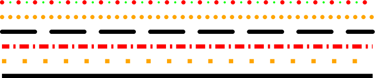
Line appearance can be varied by using PS_LINE_CAP
12.15. Specifying line attributes
A line is drawn with the texture provided by the chosen pen (Specifying pen attributes). However, depending on the module, a line also may have other attributes that can be changed in some modules. Given as modifiers to a pen specification, one or more modifiers may be appended to a pen specification. The line attribute modifiers are:
- +ooffset[u]
- Lines are normally drawn from the beginning to the end point. You can modify this behavior by requesting a gap between these terminal points and the start and end of the visible line. Do this by specifying the desired offset between the terminal point and the start of the visible line. Unless you are giving distances in Cartesian data units, please append the distance unit, u. Depending on your desired effect, you can append plot distance units (i.e., cm, inch, point; Section Length units)) or map distance units, such as km, degrees, and many other standard distance units listed in Section GMT units. If only one offset is given then it applies equally to both ends of the line. Give two slash-separated distances to indicate different offsets at the beginning and end of the line (and use 0 to indicate no offset at one end).
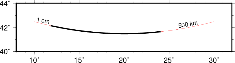
The thin red line shows an original line segment, whereas the 2-point thick pen illustrates the effect of plotting the same line while requesting offsets of 1 cm at the beginning and 500 km at the end, via -W2p+o1c/500k.
- +s
- Normally, all PostScript line drawing is implemented as a linear spline, i.e., we simply draw straight line-segments between the given data points. Use this modifier to render the line using Bezier splines for a smoother curve.
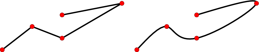
(left) Normal plotting of line given input points (red circles) via -W2p. (right) Letting the points be interpolated by a Bezier cubic spline via -W2p+s.
- +v[b|e]vspecs
- By default, lines are normally drawn from start to end. Using the +v modifier you can place arrow-heads pointing outward at one (or both) ends of the line. Use +v if you want the same vector attributes for both ends, or use +vb and +ve to specify a vector only at the beginning or end of the line, respectively. Finally, these two modifiers may both be given to specify different attributes for the two vectors. The vector specification is very rich and you may place other symbols, such as circle, square, or a terminal cross-line, in lieu of the vector head (see psxy for more details).
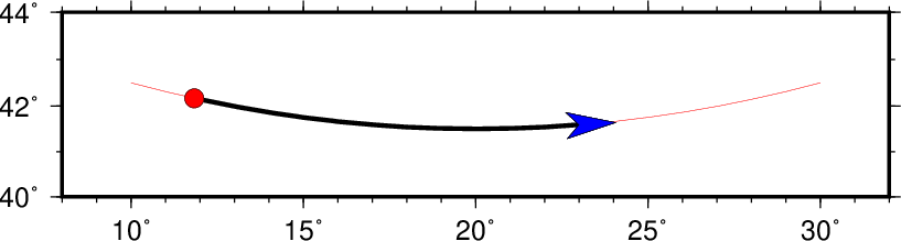
Same line as above but now we have requested a blue vector head at the end of the line and a red circle at the beginning of the line with -W2p+o1c/500k+vb0.2i+gred+pfaint+bc+ve0.3i+gblue. Note that we also prescribed the line offsets in addition to the symbol endings.
12.16. Specifying area fill attributes
Many plotting programs will allow the user to draw filled polygons or symbols. The fill specification may take two forms:
-Gfill
-Gppattern[+bcolor][+fcolor][+rdpi]
- fill:
- In the first case we may specify a gray shade (0--255), RGB color (r/g/b all in the 0--255 range or in hexadecimal #rrggbb), HSV color (hue-saturation-value in the 0--360, 0--1, 0--1 range), CMYK color (cyan/magenta/yellow/black, each ranging from 0--100%), or a valid color name; in that respect it is similar to specifying the pen color settings (see pen color discussion under Section Specifying pen attributes).
- pattern:
- The second form allows us to use a predefined bit-image pattern. pattern can either be a number in the range 1--90 or the name of a 1-, 8-, or 24-bit image raster file. The former will result in one of the 90 predefined 64 x 64 bit-patterns provided with GMT and reproduced in Chapter Predefined Bit and Hachure Patterns in GMT. The latter allows the user to create customized, repeating images using image raster files. The optional +rdpi modifier sets the resolution of this image on the page; the area fill is thus made up of a series of these “tiles”. The default resolution is 1200. By specifying upper case -GP instead of -Gp the image will be bit-reversed, i.e., white and black areas will be interchanged (only applies to 1-bit images or predefined bit-image patterns). For these patterns and other 1-bit images one may specify alternative background and foreground colors (by appending +bcolor and/or +fcolor) that will replace the default white and black pixels, respectively. Setting one of the fore- or background colors to - yields a transparent image where only the back- or foreground pixels will be painted.
Due to PostScript implementation limitations the raster images used with -G must be less than 146 x 146 pixels in size; for larger images see psimage. The format of Sun raster files [18] is outlined in Chapter GMT file formats. However, if you built GMT with GDAL then other image formats can be used as well. Note that under PostScript Level 1 the patterns are filled by using the polygon as a clip path. Complex clip paths may require more memory than the PostScript interpreter has been assigned. There is therefore the possibility that some PostScript interpreters (especially those supplied with older laserwriters) will run out of memory and abort. Should that occur we recommend that you use a regular gray-shade fill instead of the patterns. Installing more memory in your printer may or may not solve the problem!
Table fillex contains a few examples of fill specifications.
| -G128 | Solid gray |
| -G127/255/0 | Chartreuse, R/G/B-style |
| -G#00ff00 | Green, hexadecimal RGB code |
| -G25-0.86-0.82 | Chocolate, h-s-v-style |
| -GDarkOliveGreen1 | One of the named colors |
| -Gp7+r300 | Simple diagonal hachure pattern in b/w at 300 dpi |
| -Gp7+bred+r300 | Same, but with red lines on white |
| -Gp7+bred+f-+r300 | Now the gaps between red lines are transparent |
| -Gpmarble.ras+r100 | Using user image of marble as the fill at 100 dpi |
12.17. Specifying Fonts
The fonts used by GMT are typically set indirectly via the GMT defaults parameters. However, some programs, like pstext may wish to have this information passed directly. A font is specified by a comma-delimited attribute list of size, fonttype and fill, each of which is optional. The size is the font size (usually in points) but c, i or p can be added to indicate a specific unit. The fonttype is the name (case sensitive!) of the font or its equivalent numerical ID (e.g., Helvetica-Bold or 1). fill specifies the gray shade, color or pattern of the text (see section Specifying area fill attributes above). Optionally, you may append =pen to the fill value in order to draw the text outline with the specified pen; if used you may optionally skip the filling of the text by setting fill to -. If any of the attributes is omitted their default or previous setting will be retained. See Chapter PostScript fonts used by GMT for a list of all fonts recognized by GMT.
12.18. Stroke, Fill and Font Transparency
The PostScript language has no built-in mechanism for transparency. However, PostScript extensions make it possible to request transparency, and tools that can render such extensions will produce transparency effects. We specify transparency in percent: 0 is opaque [Default] while 100 is fully transparent (i.e., the feature will be invisible). As noted in section Layer PDF transparency: The -t option, we can control transparency on a layer-by-layer basis using the -t option. However, we may also set transparency as an attribute of stroke or fill (including for fonts) settings. Here, transparency is requested by appending @transparency to colors or pattern fills. The transparency mode can be changed by using the GMT default parameter PS_TRANSPARENCY; the default is Normal but you can choose among Color, ColorBurn, ColorDodge, Darken, Difference, Exclusion, HardLight, Hue, Lighten, Luminosity, Multiply, Normal, Overlay, Saturation, SoftLight, and Screen. For more information, see for instance (search online for) the Adobe pdfmark Reference Manual. Most printers and many PostScript viewers can neither print nor show transparency. They will simply ignore your attempt to create transparency and will plot any material as opaque. Ghostscript and its derivatives such as GMT’s psconvert support transparency (if compiled with the correct build option). Note: If you use Acrobat Distiller to create a PDF file you must first change some settings to make transparency effective: change the parameter /AllowTransparency to true in your *.joboptions file.
12.19. Placement of text
Many text labels placed on maps are part of the standard basemap machinery (e.g., annotations, axis labels, plot titles) and GMT automatically takes care of where these are placed and how they are justified. However, when you wish to add extra text to a plot in locations of your choice you will need to understand how we reference text to locations on the map. Figure Text justification discusses the various ways to do this.
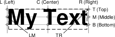
Text strings are placed on maps by associating an anchor point on the string with a reference point on the map. Nine anchor points relative to any text string may be specified by combining any of three letter codes for horizontal (Left, Center, Right) and vertical (Top, Middle, Bottom) alignments.
Notice how the anchor points refers to the text baseline and do not change for text whose letters extend below the baseline.
The concept of anchor points extends to entire text paragraphs that you may want to typeset with pstext.
A related point involves the footprint of the text and any background panel on the map. We determine the bounding box for any text string, but very often we wish to extend this box outwards to allow for some clearance between the text and the space surrounding it. Programs that allows for such clearance will let you specify offsets dx and dy that is used to enlarge the bounding box, as illustrated in Figure Text clearance.

The bounding box of any text string can be enlarged by specifying the adjustments dx and dy in the horizontal and vertical dimension. The shape of the bounding box can be modified as well, including rounded or convex rectangles. Here we have chosen a rounded rectangle, requiring the additional specification of a corner radius, r.
12.20. Color palette tables
Several programs need to relate user data to colors, shades, or even patterns. For instance, programs that read 2-D gridded data sets and create colored images or shaded reliefs need to be told what colors to use and over what z-range each color applies. Other programs may need to associate a user value with a color to be applied to a symbol, line, or polygon. This is the purpose of the color palette table (CPT). For most applications, you will simply create a CPT using the tool makecpt which will take an existing dynamic master color table and stretch it to fit your chosen data range, or use grd2cpt to build a CPT based on the data distribution in one or more given grid files. However, in rare situations you may need to make a CPT by hand or using text tools like awk or perl. Finally, if you have your own preferred color table you can convert it into a dynamic CPT and place it in your GMT user directory and it will be found and behave like other GMT master CPTs.
Color palette tables (CPT) comes in two flavors: (1) Those designed to work with categorical data (e.g., data where interpolation of values is undefined) and (2) those designed for regular, continuously-varying data. In both cases the fill information follows the format given in Section Specifying area fill attributes. The z-values in CPTs can be scaled by using the +u|Uunit mechanism. Append these modifiers to your CPT names when used in GMT commands. The +uunit modifier will scale z from unit to meters, while +Uunit does the inverse (scale z from meters to unit).
Since GMT supports several coordinate systems for color specification, many master (or user) CPTs will contain the special comment
# COLOR_MODEL = modelwhere model specifies how the color-values in the CPT should be interpreted. By default we assume colors are given as red/green/blue triplets (each in the 0-255 range) separated by slashes (model = rgb), but alternative representations are the HSV system of specifying hue-saturation-value triplets (with hue in 0-360 range and saturation and value ranging from 0-1) separated by hyphens (model = hsv), or the CMYK system of specifying cyan/magenta/yellow/black quadruples in percent, separated by slashes (model = cmyk).
12.20.1. Categorical CPTs
Categorical data are information on which normal numerical operations are not defined. As an example, consider various land classifications (desert, forest, glacier, etc.) and it is clear that even if we assigned a numerical value to these categories (e.g., desert = 1, forest = 2, etc) it would be meaningless to compute average values (what would 1.5 mean?). For such data a special format of the CPTs are provided. Here, each category is assigned a unique key, a color or pattern, and an optional label (usually the category name) marked by a leading semi-colon. Keys must be monotonically increasing but do not need to be consecutive. The format is
| key1 | Fill | [;label] |
| … | ||
| keyn | Fill | [;label] |
The Fill information follows the format given in Section Specifying area fill attributes. While not always applicable to categorical data, the background color (for key-values < \(key_1\)), foreground color (for key-values > \(key_{n}\)), and not-a-number (NaN) color (for key-values = NaN) are all defined in the gmt.conf file, but can be overridden by the statements
| B | Fillback |
| F | Fillfore |
| N | Fillnan |
12.20.2. Regular CPTs
Suitable for continuous data types and allowing for color interpolations, the format of the regular CPTs is:
| z0 | Colormin | z1 | Colormax | [A] | [;label] |
| … | |||||
| zn-2 | Colormin | zn-1 | Colormax | [A] | [;label] |
Thus, for each “z-slice”, defined as the interval between two boundaries (e.g., \(z_0\) to \(z_1\)), the color can be constant (by letting Color\(_{max}\) = Color\(_{min}\) or -) or a continuous, linear function of z. If patterns are used then the second (max) pattern must be set to -. The optional flag A is used to indicate annotation of the color scale when plotted using psscale. The optional flag A may be L, U, or B to select annotation of the lower, upper, or both limits of the particular z-slice, respectively. However, the standard -B option can be used by psscale to affect annotation and ticking of color scales. Just as other GMT programs, the stride can be omitted to determine the annotation and tick interval automatically (e.g., -Baf). The optional semicolon followed by a text label will make psscale, when used with the -L option, place the supplied label instead of formatted z-values.
As for categorical tables, the background color (for z-values < \(z_0\)), foreground color (for z-values > \(z_{n-1}\)), and not-a-number (NaN) color (for z-values = NaN) are all defined in the gmt.conf file, but can be overridden by the statements
| B | Fillback |
| F | Fillfore |
| N | Fillnan |
which can be inserted into the beginning or end of the CPT. If you prefer the HSV system, set the gmt.conf parameter accordingly and replace red, green, blue with hue, saturation, value. Color palette tables that contain gray-shades only may replace the r/g/b triplets with a single gray-shade in the 0--255 range. For CMYK, give c/m/y/k values in the 0--100 range.
A few programs (i.e., those that plot polygons such as grdview, psscale, psxy and psxyz) can accept pattern fills instead of gray-shades. You must specify the pattern as in Section Specifying area fill attributes (no leading -G of course), and only the first pattern (for low z) is used (we cannot interpolate between patterns). Finally, some programs let you skip features whose z-slice in the CPT file has gray-shades set to -. As an example, consider
| 30 | p16+r200 | 80 | - |
| 80 | - | 100 | - |
| 100 | 200/0/0 | 200 | 255/255/0 |
| 200 | yellow | 300 | green |
where slice 30 < z < 80 is painted with pattern # 16 at 200 dpi, slice 80 < z < 100 is skipped, slice 100 < z < 200 is painted in a range of dark red to yellow, whereas the slice 200 < z < 300 will linearly yield colors from yellow to green, depending on the actual value of z.
Some programs like grdimage and grdview apply artificial illumination to achieve shaded relief maps. This is typically done by finding the directional gradient in the direction of the artificial light source and scaling the gradients to have approximately a normal distribution on the interval [-1,+1]. These intensities are used to add “white” or “black” to the color as defined by the z-values and the CPT. An intensity of zero leaves the color unchanged. Higher values will brighten the color, lower values will darken it, all without changing the original hue of the color (see Chapter Color Space: The Final Frontier for more details). The illumination is decoupled from the data grid file in that a separate grid file holding intensities in the [-1,+1] range must be provided. Such intensity files can be derived from the data grid using grdgradient and modified with grdhisteq, but could equally well be a separate data set. E.g., some side-scan sonar systems collect both bathymetry and backscatter intensities, and one may want to use the latter information to specify the illumination of the colors defined by the former. Similarly, one could portray magnetic anomalies superimposed on topography by using the former for colors and the latter for shading.
12.20.3. Master (dynamic) CPTs
The CPTs distributed with GMT are dynamic. This means they have several special properties that modify the behavior of programs that use them. All dynamic CPTs are normalized in one of two ways: If a CPT was designed to behave differently across a hinge value (e.g., a CPT designed specifically for topographic relief may include a discontinuity in color across the coastline at z = 0), then the CPT’s z-values will range from -1, via 0 at the hinge, to +1 at the other end. The hinge value is specified via the special comment
# HINGE = <hinge-value>CPTs without a hinge are instead normalized with z-values from 0 to 1. Dynamic CPTs will need to be stretched to the user’s preferred range, and there are two modes of such scaling: Some CPTs designed for a specific application (again, the topographic relief is a good example) have a default range specified in the master table via the special comment
# RANGE = <zmin/zmax>and when used by applications the normalized z-values will be stretched to reflect this natural range. In contrast, CPTs without a natural range are instead stretched to fit the range of the data in question (e.g., a grid’s range). Exceptions to these rules are implemented in the two CPT-producing modules makecpt and grd2cpt, both of which can read dynamic CPTs and produce static CPTs satisfying a user’s specific range needs. These tools can also read static CPTs where the new range must be specified (or computed from data), reversing the order of colors, and even isolating a section of an incoming CPT. Here, makecpt can be told the range of compute it from data tables while grd2cpt can derive the range from one or more grids.
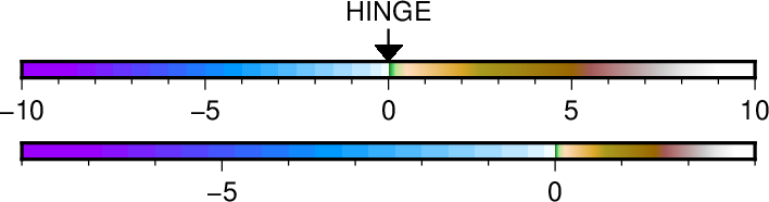
The top color bar is a dynamic master CPT (here, globe) with a hinge at sea level and a natural range from -10,000 to +10,000 meters. However, our data range is asymmetrical, going from -8,000 meter depths up to +3,000 meter elevations. Because of the hinge, the two sides of the CPT will be stretched separately to honor the desired range while utilizing the full color range.
12.20.4. Cyclic (wrapped) CPTs
Any color table you produce can be turned into a cyclic or wrapped color table. This is performed by adding the -Ww option when running makecpt or grd2cpt. This option simply adds the special comment
# CYCLICto the color table and then GMT knows that when looking up a color from a z value it will remove an integer multiple of the z-range represented by the color table so that we are always inside the range of the color table. This means that the fore- and back-ground colors can never be activated. Wrapped color tables are useful for highlighting small changes.
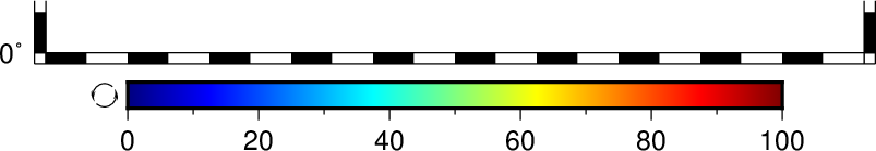
Cyclic color bars are indicated by a cycle symbol on the left side of the bar.
12.20.5. Manipulating CPTs
There are many ways to turn a master CPT into a custom CPT that works for your particular data range. The tools makecpt and grd2cpt allow several types of transformations to take place:
- You can reverse the z-direction of the CPT using option -Iz. This is useful when your data use a different convention for positive and negative (e.g., perhaps using positive depths instead of negative relief).
- You can invert the order of the colors in the CPT using option -Ic. This is different from the previous option in that only the colors are rearranged (it is also possible to issue -Icz to combine both effects.)
- You can select just a subset of a master CPT with -G, in effect creating a modified master CPT that can be scaled further.
- Finally, you can scale and translate the (modified) master CPT range to your actual data range or a sub-range thereof.
The order of these transformations is important. For instance, if -Iz is given then all other z-values need to be referred to the new sign convention. For most applications only the last transformation is needed.
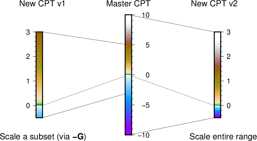
Examples of two user CPTs for the range -0.5 to 3 created from the same master. One (left) extracted a subset of the master before scaling while the other (right) used the entire range.
12.21. The Drawing of Vectors
GMT supports plotting vectors in various forms. A vector is one of many symbols that may be plotted by psxy and psxyz, is the main feature in grdvector, and is indirectly used by other programs. All vectors plotted by GMT consist of two separate parts: The vector line (controlled by the chosen pen attributes) and the optional vector head(s) (controlled by the chosen fill). We distinguish between three types of vectors:
- Cartesian vectors are plotted as straight lines. They can be specified by a start point and the direction and length (in map units) of the vector, or by its beginning and end point. They may also be specified giving the azimuth and length (in km) instead.
- Circular vectors are (as the name implies) drawn as circular arcs and can be used to indicate opening angles. It accepts an origin, a radius, and the beginning and end angles.
- Geo-vectors are drawn using great circle arcs. They are specified by a beginning point and the azimuth and length (in km) of the vector, or by its beginning and end point.
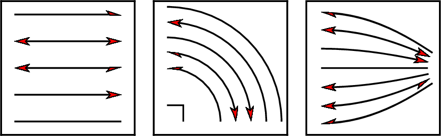
Examples of Cartesian (left), circular (middle), and geo-vectors (right) for different attribute specifications. Note that both full and half arrow-heads can be specified, as well as no head at all.
There are numerous attributes you can modify, including how the vector should be justified relative to the given point (beginning, center, or end), where heads (if any) should be placed, if the head should just be the left or right half, if the vector attributes should shrink for vectors whose length are less than a given cutoff length, and the size and shape of the head. These attributes are detailed further in the relevant manual pages.
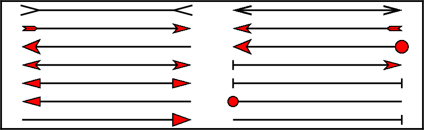
Examples of different vector heads and attributes. The default is the standard triangular arrow head, which can be modified by adjusting the apex angle [30] or changing its shape via the MAP_VECTOR_SHAPE setting. Other vector heads are the circle (c), the terminal line (t), the arrow fin (i) and the plain head (A) and tail (I); the last two are line-drawings only and cannot be filled.
12.22. Character escape sequences
For annotation labels or text strings plotted with pstext, GMT provides several escape sequences that allow the user to temporarily switch to the symbol font, turn on sub- or superscript, etc., within words. These conditions are toggled on/off by the escape sequence @x, where x can be one of several types. The escape sequences recognized in GMT are listed in Table escape. Only one level of sub- or superscript is supported. Note that under Windows the percent symbol indicates a batch variable, hence you must use two percent-signs for each one required in the escape sequence for font switching.
| @~ | Turns symbol font on or off |
| @+ | Turns superscript on or off |
| @- | Turns subscript on or off |
| @# | Turns small caps on or off |
| @_ | Turns underline on or off |
| @%fontno% | Switches to another font; @%% resets to previous font |
| @:size: | Switches to another font size; @:: resets to previous size |
| @;color; | Switches to another font color; @;; resets to previous color |
| @! | Creates one composite character of the next two characters |
| @@ | Prints the @ sign itself |
Shorthand notation for a few special European characters has also been added (for others you must use the full octal code):
| Code | Effect | Code | Effect |
|---|---|---|---|
| @E | Æ | @e | æ |
| @O | Ø | @o | ø |
| @A | Å | @a | å |
| @C | Ç | @c | ç |
| @N | Ñ | @n | ñ |
| @U | Ü | @u | ü |
| @s | ß | @i | í |
PostScript fonts used in GMT may be re-encoded to include several accented characters used in many European languages. To access these, you must specify the full octal code \xxx allowed for your choice of character encodings determined by the PS_CHAR_ENCODING setting described in the gmt.conf man page. Only the special characters belonging to a particular encoding will be available. Many characters not directly available by using single octal codes may be constructed with the composite character mechanism @!.
Some examples of escape sequences and embedded octal codes in GMT strings using the Standard+ encoding:
2@~p@~r@+2@+h@-0@- E\363tv\363s = 2\(\pi r^2h_0\) Eötvös10@+-3 @Angstr@om = 10\(^{-3}\) ÅngstrømStresses are @~s@~@+*@+@-xx@- MPa = Stresses are \(\sigma^{*}_{xx}\) MPaSe@nor Gar@con = Señor GarçonM@!\305anoa stra@se = Manoa straßeA@\#cceleration@\# (ms@+-2@+) = ACCELERATIONThe option in pstext to draw a rectangle surrounding the text will not work for strings with escape sequences. A chart of characters and their octal codes is given in Chapter Chart of Octal Codes for Characters.
12.23. Plot embellishments
Apart from visualizing your data sets, GMT maps can also be embellished in several ways. The 8 embellishments currently available are
- Map scale showing the true scale at some location(s) on the map.
- Directional rose showing true north and other cardinal directions.
- Magnetic rose showing magnetic north and declination deviations.
- Color bar relating the colors of your image to the data values.
- Map legend showing the meaning of the symbols on your map.
- Image overlay of raster images or EPS figures (e.g., institutional logos, photos, etc.).
- GMT logo overlay.
- Map insert showing perhaps the location of your detailed area in a regional or global context.
Each of these features share a common system for specifying the location on the plot where the feature will be placed. They also share a common way for specifying the placement of a rectangular panel behind the feature (to provide a uniform background, for instance). Thus, before we discuss the different features in more detail we will first review the “reference point/anchor point” system used by GMT to specify such locations in relation to the underlying map, and then discuss the background panel attribute settings.
12.23.1. Reference and anchor point specification
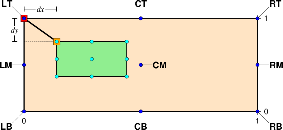
The placement of a map feature (here represented by a green rectangle) in relation to the underlying map. The nine named reference points (blue circles) on the map perimeter (and center) can be used to specify a location. Using the same system of nine points on the map feature (cyan circles) we select one of these as our anchor point (here TL, indicated by the orange square). The anchor point can optionally be shifted away from the reference point by an amount dx/dy in the direction implied by the anchor point (in this case to the top and left), yielding the adjusted anchor point (red square). The feature is then placed such that its adjusted anchor point matches the reference point.
Placing a feature on the map means selecting a reference point somewhere on the map, an anchor point somewhere on the feature, and then positioning the feature so that the two points overlap. It may be helpful to consider the analog of a boat dropping an anchor: The boat navigates to the reference point and then, depending on where on the boat the anchor is located, moves so that the anchor connection point overlies the reference point, then drops the anchor. There are four different ways to specify the reference point on a map, allowing for complete freedom to select any location inside or outside the map. The reference point syntax is [g|j|J|n|x]refpoint; the five codes g|j|J|n|x refer to the five ways:
- [g] Specify refpoint using data coordinates, e.g., the longitude and latitude of the reference point. This mechanism is useful when you want to tie the location of the feature to an actual point best described by data coordinates. An example of such a reference point might be g135W/20N.
- [j] Specify refpoint using one of the nine justification codes, equivalent to the justification codes for placing text strings in pstext. This mechanism is illustrated in the figure above and is the preferred mechanism when you just want to place the feature inside the basemap at one of the corners or centered at one of the sides (or even smack in the middle). Justification codes are a combination of a horizontal (L, C, R) and a vertical (T, M, B) code. An example of such a reference point might be jTL. When used, the anchor point on the map feature will default to the same justification, i.e., TL in this example.
- [J] This is the same as j except it implies that the default anchor point is the mirror opposite of the justification code. Thus, when using JTL, the anchor point on the map feature will default to BR. This is practical for features that are drawn outside of the basemap (like color bars often are).
- [x] Specify refpoint using plot coordinates, i.e., the distances in inches, centimeters, or points from the lower left plot origin. This mechanism is preferred when you wish to lay out map features using familiar measurements of distance from origins. An example of such a reference point might be x2.75i/2c.
- [n] Specify refpoint using normalized coordinates, i.e., fractional coordinates between 0 and 1 in both the x and y directions. This mechanism avoids units and is useful if you want to always place features at locations best referenced as fractions of the plot dimensions. An example of such a reference point might be n0.2/0.1.
If no code is specified we default to x.
With the reference point taken care of, it is time to select the anchor point. While the reference point selection gives unlimited flexibility to pick any point inside or outside the map region, the anchor point selection is limited to the nine justification points discussed for the j reference point code above. Add +janchor to indicate which justification point of the map feature should be co-registered with the chosen reference point. If an anchor point is not specified then it defaults to the justification point set for the reference point (if jcode was used to set it), or to the mirror opposite of the reference point (if Jcode was used); with all other specifications of the reference point, the anchor point takes on the default value of MC (for map rose and map scale) or BL (all other map features). Adding +janchor overrules those defaults. For instance, +jTR would select the top right point on the map feature as the anchor.
It is likely that you will wish to offset the anchor point away from your selection by some arbitrary amount, particularly if the reference point is specified with j|Jcode. Do so with +odx[/dy], where dy equals dx if it is not provided. These increments are added to the projected plot coordinates of the anchor point, with positive values moving the reference point in the same direction as the 2-character code of the anchor point implies. Finally, the adjusted anchor point is matched with the reference point.
Take for example an anchor point on the top left of the map feature, either by using a reference point jTL, or JBR, or explicitly setting +jTL. Then +o2c/1c will move the anchor point 2 cm left and 1 cm above the top left corner of the map feature. In other words, the top left corner of the map feature will end up 2 cm to the right and 1 cm below the selected reference point.
Similarly +jBR will align the bottom right corner of the map feature, and +o2c/1c will offset it 2 cm to the left and 1 cm up. When using middle (M) or center (C) justifications, to offset works the same way as bottom (B) or left (L), respectively, i.e., moving the map feature up or to the right.
12.23.2. The background panel
For most maps you will wish to place a background panel of uniform color behind any of the map features you plan to add. Because the panel is linked to the map feature you have selected, the parameters such as location and dimensions are handled automatically. What remains is to specify the attributes of the panel. Typically, panels settings are given via a module’s -F option by appending one or more modifiers. Here is a list of the attributes that are under your control:
- Color or pattern. You specify the fill you want with +gfill [Default is no fill]. For instance, paint the panel yellow with +gyellow.
- Panel frame pen. Turn on the frame outline with +p, using the pen defined via MAP_FRAME_PEN. You may override this choice with +ppen [Default is no outline]. A very bold red outline might look like +pthick,red.
- Rounded versus straight rectangle. By specifying a corner radius with +rradius you can round the corners [Default is no rounding]. Here is a 0.2-inch radius rounding: +r0.2i.
- Inner frame. A secondary, inner frame outline may be added as well with the modifier +i[[gap/]pen]. The default pen is given by MAP_DEFAULT_PEN, with a default gap between the outer and inner frames of 2 points. Add arguments to override these defaults, such as +i0.1c/thin,dashed to get a thin, dashed inner frame offset by 0.1 cm from the main (outer) frame.
- Panel clearance. The panel’s dimensions are automatically determined from knowledge of its contents. However, it is sometimes required to add some extra clearance around most or all sides, and you can do so with +c[clearance], with a 4-point clearance being the default. Add one (uniform), two (different horizontal and vertical clearances), or four (separate for sides west, east, south, and north) clearances, separated by slashes. For instance, to add a 1 cm clearance in x and 5 points in y, use +c1c/5p.
- Drop-down shadow. Append +s to simulate a gray shadow cast toward the southeast. You may append [dx/dy/][shade] to change the shade color and the offset of the shade [Default is 4p/-4p/gray50]. If happy with the placement but desiring a dark blue shadow, add +sdarkblue.

A map panel is a rectangular background placed behind any of the map features. It has several attributes that can be changed with panel option modifiers. The light green rounded rectangle was specified with -F+glightgreen+r, while the white panel on the lower right was set with -F+p1p+i+s+gwhite+c0.1i (we added a light dashed box to indicate the effect of the clearance setting).
12.23.3. Placing map scales
Traditionally, a map scale is added to maps for helping the reader understand the particular scale used for this map, i.e., it portrays the relationship between actual distances on the Earth (in km, miles, meters, etc.) and distances on the map (in cm, inches, points). Depending on the map projection the map scale will vary continuously but may be constant along a line of latitude (e.g., Mercator projection). Thus, in placing the map scale on the map there are two locations involved: (1) The reference point where the map scale’s anchor should be pinned, and (2) the projection point where the scale is computed and thus where the map scale is true. Map scales can be plotted by psbasemap or pscoast, and in addition to the the required refpoint and anchor arguments specifying where the scale should be placed there are both required and optional modifiers. These are given via these modules’ -L option. Here is a list of the attributes that is under your control:
- Scale bar length. Required modifier is given with +wlength[unit], where unit is one of the recognized distance units. An example might be +w250n for a bar representing 250 nautical miles at the map scale origin.
- Map scale origin. Required modifier given with +c[slon/]slat, where the longitude of the scale origin is optional for projections with constant scale along parallels. For a Mercator projection it may look like +c30N while an oblique projection may need +c100W/23N, for instance.
- Fancy scale bar. By default a plain-looking scale bar is plotted. For a free upgrade to a fancier bar, append +f. The fancier bar is, well, a bit fancier.
- Scale label. Turn on scale labels with +l. By default, the scale label is initialized to equal the distance unit name. Use the +llabel argument to supply your own scale label, such as +l”Distances at Equator”.
- Scale label alignment. The default alignment is on top of the bar [+at], but you can change this by selecting another alignment by appending them to the +a modifier, including bottom, left, or right. Here, +ab would align on the bottom of the scale.
- Append distance unit. For the fancy scale, adding +u will append the distance unit specified with +w to all distance annotations along the bar, while for the plain scale it will replace the default scale label with the unit abbreviation.
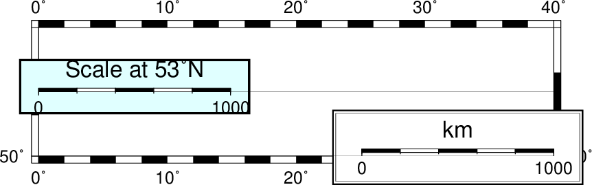
Example of two map scales for a Mercator projection evaluated at 53 degrees north. The left-most scale was placed with -LjML+c53+w1000k+f+l”Scale at 53\232N” while the scale on the right was placed with -LjBR+c53+w1000k+l+f.
Note that for the purpose of anchor justification (+j) the footprint of the map scale is considered the rectangle that contains the scale and all selected labels and annotations, i.e., the map scale’s bounding box.
12.23.4. Placing directional map roses
Map roses showing the cardinal directions of a map help the reader orient themselves, especially for oblique projections where north-south is not vertically aligned. However, these roses also have ornamental value and can be used on any map projection. As for map scales, a directional map rose is added with psbasemap or pscoast and selected by the -Td option. This option accepts the reference point where the map rose’s anchor should be pinned. In addition to the required refpoint and anchor arguments (and their standard modifiers discussed earlier) there is one required and two optional modifiers. The required modifier sets the side:
- Size of map rose. Use +wsize to specify the full width and height of the rose. A 3 cm rose would require +w3c.
The next two modifiers are optional:
- Cardinal points. By default only the four cardinal points (W, E, S, N) are included in the rose. You can extend that with the +flevel modifier, where level is 1 [Default], 2, or 3. Selecting 2 will include the two intermediate orientations NW-SE and NE-SW, while 3 adds the four additional orientations WNW-ESE, NNW-SSE, NNE-SSW, and ENE-WSW.
- Add labels. Do so with +l, which places the current one-letter codes for west, east, south, and north at the four cardinal points. These letters depend on the setting of GMT_LANGUAGE and for the default English we use W, E, S, N, respectively. You can replace these labels with four custom labels via +lw,e,s,n, i.e., four comma-separated labels in the specified order. You can exclude any of the cardinal points from being labeled by giving no label in the corresponding order. E.g., +l”,,Down,Up” would write Down and Up at the south and north cardinal point, respectively. Note that for the plain directional rose only the north annotation will be placed.
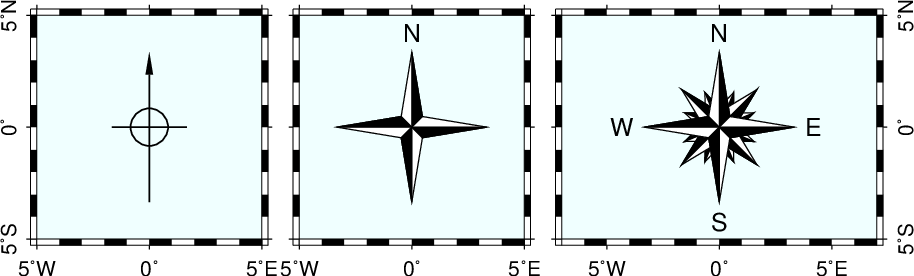
Plain and fancy directional map roses. (left) Bare-bones plain rose showing arrow towards north and a cross indicating the cardinal directions, specified by -Tdg0/0+w1i. (middle) Fancy rose obtained by adding +f and +l,,,N to get the north label. (right) Fancy directional rose at level 3 with labels by adding +f3+l.
12.23.5. Placing magnetic map roses
Map roses showing the magnetic directions of a map are useful when magnetic data are presented, or when declinations are significantly nonzero. However, as for directional roses the magnetic rose also has ornamental value. The magnetic rose consists of two concentric angular scales: The first (outer) ring shows directional angles while the second (inner) ring is optional and portrays the magnetic directions, which differ for nonzero declination. As for style, the two-ring rose looks a bit like a standard compass. As for directional roses, a magnetic map rose is added with psbasemap or pscoast and selected by the -Tm option. As for other features, append the required reference point where the magnetic map rose’s anchor should be pinned. There is one required and several optional modifiers. First up is the size:
- Specify size of map rose. Use +wsize to specify the full width of the rose. A 3 cm rose would imply +w3c.
The remaining modifiers are optional:
- Specify Declination. To add the inner angular scale, append ddec[/dlabel], where dec is the declination value in decimal or ddd:mm:ss format, and dlabel is an optional string that replaces the default label (which is “d = dec”, with d being a Greek delta and we format the specified declination). Append ddec/- to indicate you do not want any declination label. As an example, consider d11/”Honolulu declination”.
- Draw the secondary (outer) ring outline. Normally it is not drawn, but you can change that by appending +ppen. For instance, adding +pthin will draw the ring with the selected thin pen.
- Add labels. As for directional roses you do so with +l, which places the current one-letter codes for west, east, south, and north at the four cardinal points. These letters depend on the setting of GMT_LANGUAGE and for the default English we use W, E, S, N, respectively. You can replace these labels with four custom labels via +lw,e,s,n, i.e., four comma-separated labels in the specified order. You can exclude any of the cardinal points from being labeled by giving no label in the corresponding order. E.g., +l”,,Down,Up” would write Down and Up at the south and north cardinal point, respectively.
- Draw the primary (inner) ring outline. It is also not normally drawn; change that by appending +ipen. For instance, adding +ithin,blue will draw the ring with the selected thin, blue pen.
- Set annotation, tick and grid intervals. Each ring has a default annotation [30], tick [5], and grid [1] interval (although here “grid interval” is just a finer tick interval drawn at half tickmark length). Adjust these three intervals with +tintervals. If you selected +d then you must supply two sets of such intervals (i.e., 6 comma-separated values), where the first (primary) set refers to the declination-adjusted ring and the second (secondary) set refers to the directional (outer) ring. If only three intervals are given then we assume you want the same intervals for both rings. As an example, to annotate every 90 degrees and tick every 15 and 5 degrees, add +t90/15/5.
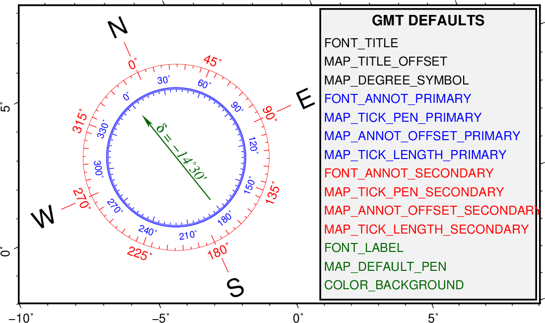
Magnetic direction map rose. This symbol is quite complicated and has many items whose attributes are in part controlled by GMT defaults parameters and in part by the above modifiers. The color-coded legend indicates which parameters controls the font, pen, or color of the correspond item of the rose. This rose was specified by -Tmg-2/0.5+w2.5i+d-14.5+t45/10/5+i0.25p,blue+p0.25p,red+l+jCM. See gmt.conf for more details on the default parameters.
12.23.6. Placing color scale bars
Color scale bars are used in conjunction with color-coded surfaces, symbols, lines, or even text, to relate the chosen color to a data value or category. For instance, color images of topography or other gridded data will need a mechanism for users to decode what the colors represent. Typically, we do this by adding a color scale bar on the outside (or inside) of the map boundaries. The module psscale places the color scale bar, with location and size determined by the -D attributes. As for other map features we must specify the reference and anchor points and any adjustments to them, then supply suitable required and optional modifiers:
- Give dimensions of color bar. Use +wlength/width to specify the full width and height of the bar. For instance, a 10 cm long bar of height 0.5 cm would imply +w10c/0.5c.
- Set orientation of color bar. By default, we place a vertically aligned bar. Select a horizontal bar by adding +h.
- Specify color bar label alignment. By default we place the chosen annotations, scale (i.e., x-axis) label and unit (i.e., y-axis) label on the opposite side of the color scale bar anchor point. Change this with +m and append any combination of a, l, or u to flip the annotations or labels to the opposite side. Append c to plot vertical labels as column text (this cannot be used with +h, obviously).
- Extend the color bar. You can use the +e modifier to add sidebar triangles for displaying the current back- and foreground colors. Append b (background) or f (foreground) to get the implied side only [Default is both]. Optionally, append triangle height [Default is half the bar width].
- Add missing data key. Append +n to draw a rectangle with the current NaN color and label it NaN. Optionally, append a replacement text. One example might be +n”No data”.
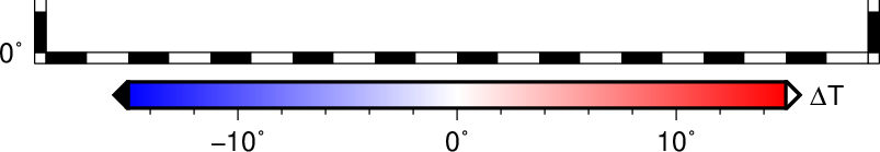
Color bar placed beneath a map (here truncated). We extended the bar to show background and foreground colors, and used the frame-annotation machinery to add labels. The bar was placed with -DJBC+o0/0.35i+w4.5i/0.1i+h.
12.23.7. Placing map legends
Adding map legends is the standard way to communicate what various symbols placed on your map represent. For instance, you may use this mechanism to convey the information that circles are earthquake locations, triangles are places where you ate Thai food, and dashed lines indicate some sort of gang-land demarkation line that you should not cross without paying the locals due respect. Map legends are placed by the module pslegend, with location and size determined by the various -D attributes. We must again specify the reference and anchor points and any adjustments to them first, then supply suitable required and optional modifiers:
- Give legend dimensions. You must specify the required legend width, while legend height is optional and if not given is computed based on the contents of the legend. The syntax is therefore +wwidth[/height] in your desired plot units. Thus, +w12c sets the legend width as 12 cm but the hight will become whatever is needed to contain the information.
- Set line-spacing. You may optionally specify the line-spacing used for the setting of the legend. The legend will typically consist of several lines that may or may not contain text, but the spacing between these lines are controlled by the chosen line-spacing factor times the current primary annotation font setting, i.e., FONT_ANNOT_PRIMARY. The default line spacing factor is 1.1; change this with +llinefactor.
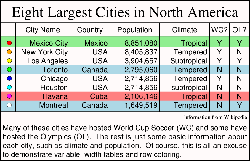
Example of a map legend placed with pslegend. Apart from the placement and dimensions discussed here, pslegend reads macro commands that specifies each item of the legend, including colors, widths of columns, the number of columns, and presents a broad selection of items. Here, we simply used -Dx0/0+w5.6i+jBL.
12.23.8. Placing raster and EPS images on maps
When preparing posters for meetings one will often need to include the organization’s logo, which may be available to you as an Encapsulated PostScript File (EPS) or as a raster image, such as PNG or JPG. At other times, you may wish to place photos or other raster images on your map. The module psimage can help with this, and like the other map feature placements it requires a reference point and its optional adjustments via the -D option. In addition, we require one (of two) modifiers to determine the image size.
- Specify image width. This is a required modifier and is set via +wwidth[/height]. If height is specified as 0 then we compute the height from width and the aspect ratio of the image, for instance +w4c/0. If width is negative the we use its absolute value as width but interpolate the image in PostScript to the device resolution.
- Specify image resolution. For raster images (not EPS) you may instead specify the size of the plotted image by specifying its resolution in dots per inch, via +rdpi. The actual size of the images is then controlled by its number of pixels times the dpi.
- Enable image replication. For raster images (not EPS) you may optionally append +nnx[/ny] to indicate that you want the source image to be replicated that many times in the two directions, resulting in a tiling of the map using the selected image. This may be useful in conjunction with an active clip path set by psclip.

Placement of EPS and raster images. (left) The US National Science Foundation (NSF) has generously funded the development of GMT and their JPG logo is reproduced here via -DjML+w1.5i+o0.1i. (right) The School of Ocean and Earth Science and Technology at the University of Hawaii at Manoa hosts the gmt server and its EPS logo is shown via -DjMR+o0.1i+w2i.
12.23.9. Placing a GMT logo on maps
It is possible to overlay the GMT logo on maps as well, using the module gmtlogo. Like other features it requires reference and anchor points and their optional adjustments via the -D option. In addition, we require one modifier to set the logo’s size.
- Specify logo width. This is a required modifier and is set via +wwidth. The height is automatically set (it is half the width). To place a 5 cm wide GMT logo, append +w5c.

Placement of the GMT logo. The logo itself only has a size modifier but the gmtlogo module allows additional attributes such as a background map panel.
12.23.10. Placing map inserts
Our final map embellishment is the map insert. A map insert may appear to be the easiest feature to add since it only consists of an empty map panel. What you put in this panel is up to you (and we will show some examples). However, unlike the other map features there are two ways to specify the placement of the map insert. The first is the standard way of specifying the reference and anchor points and the insert dimensions, while the second specifies a subregion in the current plot that should be designated the map insert area. Depending on the map projection this may or may not be a rectangular area. Map inserts are produced by the module psbasemap via the -D option. Unless you use the reference point approach you must first append xmin/xmax/ymin/ymax[+r][+uunit], where the optional unit modifier +u indicates that the four coordinates to follow are projected distances (e.g., km, miles). If the unit modifier is missing then we assume the coordinates are map coordinates (e.g., geographic west, east, south, and north). For oblique projections you may wish to specify the domain using the lower-left and upper-right coordinates instead (similar to how the -R option works), by adding +r. Some optional modifiers are available:
- Set insert size. If you specified a reference point then you must also specify the insert dimensions with the +wwidth[unit][/height[unit]], where height defaults to width if not given. Append the unit of the dimensions, which may be distance units such as km, feet, etc., and the map projection will be used to determine insert dimensions on the map. For instance, +w300k/200k is a 300x200 km region (which depends on the projection) while +w5c is a 5cm square box.
- Save the location and dimensions. For all but the simplest of map inserts you will need to know the exact location of the resulting insert and its dimensions. For instance, if you specified the insert using the TR anchor point and a width and height of 100 km you will need to know what this means in terms of positions on the map in plot units. In terms of the modifiers this would be jTR+w100k. Running psbasemap in verbose mode will provide this information and you can use it accordingly. However, for users who wish to script this automatically you can use +sfile to save this information in a file that your script can ingest and act upon. The file contains a single record with the four tab-separated values x0 y0 width height in the current plot units [cm], where x0 y0 refers to the lower-left point on the insert. See the figure caption for an example.
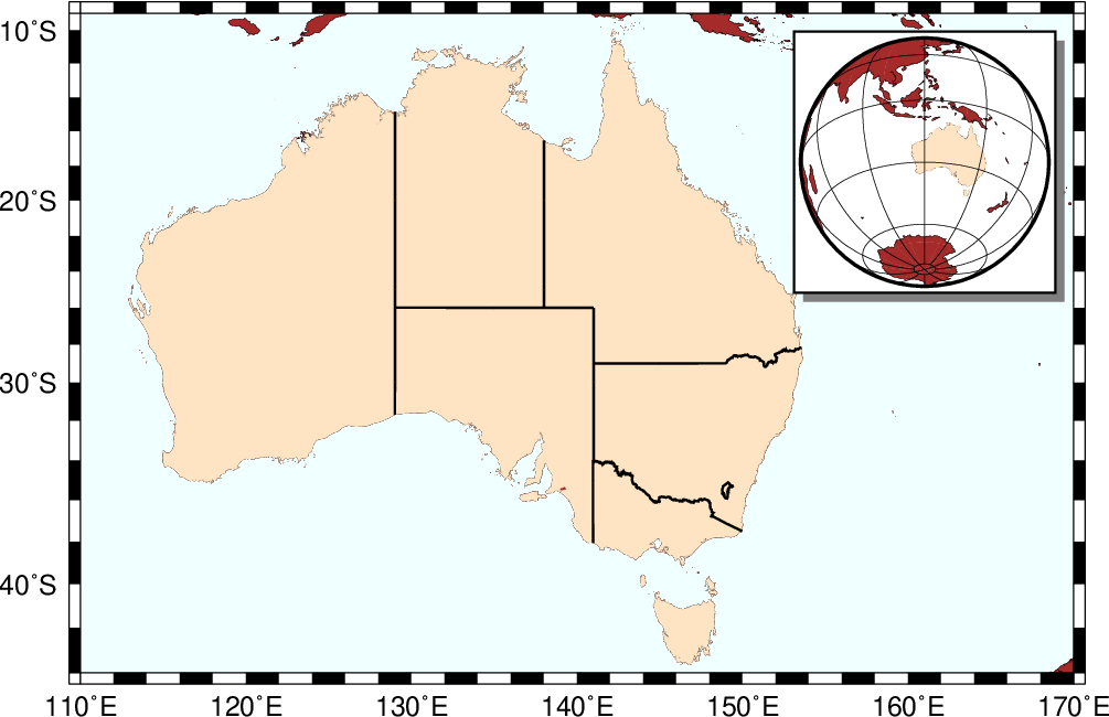
Demonstration of how a map insert may be used to place a global overview map as an insert in a regional map. Main map shows the regional area of Australia. We place an insert in the upper right area with -DjTR+w1.5i+o0.15i+stmp and then read in the coordinates of the lower-right corner of the insert and its dimension with UNIX (“read x0 y0 w h < tmp”). Knowing the placement (we know the size of the circular global map) we can correctly position it in the insert with -X$x0 and -Y$y0. See Example (44) Map inserts for more details.
12.24. Grid file format specifications
GMT has the ability to read and write grids using more than one grid file format (see Table grdformats for supported format and their IDs). For reading, GMT will automatically determine the format of grid files, while for writing you will normally have to append =ID to the filename if you want GMT to use a different format than the default. The automatic reading procedure follows an heuristic where certain formats are tentatively decoded with GMT internal drivers and if they fail than we resort to use the GDAL library to do the readings. This normally works pretty well but in case of failure (e.g. a GMT driver failed to read binary file with a separate header that also could have been stored in an ASCII file with embed header) the user should explicitly try to force a reading via GDAL. That is, to append a =gd suffix to file name.
By default, GMT will create new grid files using the nf format; however, this behavior can be overridden by setting the IO_GRIDFILE_FORMAT defaults parameter to any of the other recognized values (or by appending =ID).
GMT can also read netCDF grid files produced by other software packages, provided the grid files satisfy the COARDS and Hadley Centre conventions for netCDF grids. Thus, products created under those conventions (provided the grid is 2-, 3-, 4-, or 5-dimensional) can be read directly by GMT and the netCDF grids written by GMT can be read by other programs that conform to those conventions. Three such programs are ncview, Panoply, and ncBrowse ; others can be found on the netCDF website. Note that although many additional programs can read netCDF files, some are unable to read netcdf 4 files (if data compression has been applied).
In addition, users with some C-programming experience may add their own
read/write functions and link them with the GMT library to extend the
number of predefined formats. Technical information on this topic can be
found in the source file gmt_customio.c. Users who are considering this approach
should contact the GMT team.
| ID | Explanation |
|---|---|
| GMT 4 netCDF standard formats | |
| nb | GMT netCDF format (8-bit integer, COARDS, CF-1.5) |
| ns | GMT netCDF format (16-bit integer, COARDS, CF-1.5) |
| ni | GMT netCDF format (32-bit integer, COARDS, CF-1.5) |
| nf | GMT netCDF format (32-bit float, COARDS, CF-1.5) |
| nd | GMT netCDF format (64-bit float, COARDS, CF-1.5) |
| GMT 3 netCDF legacy formats | |
| cb | GMT netCDF format (8-bit integer, depreciated) |
| cs | GMT netCDF format (16-bit integer, depreciated) |
| ci | GMT netCDF format (32-bit integer, depreciated) |
| cf | GMT netCDF format (32-bit float, depreciated) |
| cd | GMT netCDF format (64-bit float, depreciated) |
| GMT native binary formats | |
| bm | GMT native, C-binary format (bit-mask) |
| bb | GMT native, C-binary format (8-bit integer) |
| bs | GMT native, C-binary format (16-bit integer) |
| bi | GMT native, C-binary format (32-bit integer) |
| bf | GMT native, C-binary format (32-bit float) |
| bd | GMT native, C-binary format (32-bit float) |
| Miscellaneous grid formats | |
| rb | SUN raster file format (8-bit standard) |
| rf | GEODAS grid format GRD98 (NGDC) |
| sf | Golden Software Surfer format 6 (32-bit float) |
| sd | Golden Software Surfer format 7 (64-bit float) |
| af | Atlantic Geoscience Center AGC (32-bit float) |
| ei | ESRI Arc/Info ASCII Grid Interchange format (ASCII integer) |
| ef | ESRI Arc/Info ASCII Grid Interchange format (ASCII float) |
| gd | Import/export via GDAL [19] |
Because some formats have limitations on the range of values they can store it is sometimes necessary to provide more than simply the name of the file and its ID on the command line. For instance, a native short integer file may use a unique value to signify an empty node or NaN, and the data may need translation and scaling prior to use. Therefore, all GMT programs that read or write grid files will decode the given filename as follows:
name[=ID[+sscale][+ooffset][+ninvalid]]
where anything in brackets is optional. If you are reading a grid then no options are needed: just continue to pass the name of the grid file. However, if you write another format you must append the =ID string, where ID is the format code listed above. In addition, should you want to (1) multiply the data by a scale factor, and (2) add a constant offset you must append the +sscale and +ooffset modifiers. Finally, if you need to indicate that a certain data value should be interpreted as a NaN (not-a-number) you must append +ninvalid modifier to file name. You may the scale as a for auto-adjusting the scale and/or offset of packed integer grids (=ID+sa is a shorthand for =ID+sa+oa).
Some of the grid formats allow writing to standard output and reading from standard input which means you can connect GMT programs that operate on grid files with pipes, thereby speeding up execution and eliminating the need for large, intermediate grid files. You specify standard input/output by leaving out the filename entirely. That means the “filename” will begin with “=ID”. Note, that the netCDF format does not allow piping.
Everything looks clearer after a few examples:
- To write a native binary float grid file, specify the name as
my_file.f4=bf. - To read a native short integer grid file, multiply the data by 10 and
then add 32000, but first let values that equal 32767 be set to NaN,
use the filename
my_file.i2=bs+s10+o32000+n32767. - To read a Golden Software “surfer” format 6 grid file, just pass the
file name, e.g.,
my_surferfile.grd. - To read a 8-bit standard Sun raster file (with values in the 0--255
range) and convert it to a 1 range, give the name as
rasterfile=rb+s7.84313725e-3+o-1(i.e., 1/127.5). - To write a native binary short integer grid file to standard output
after subtracting 32000 and dividing its values by 10, give filename
as
=bs+s0.1+o-3200. - To write an 8-bit integer netCDF grid file with an auto-adjusted
offset, give filename as
=nb+oa. - To read a short integer .bil grid file stored in binary and and force
the reading via GDAL, add suffix =gd as in
n45_e008_1arc_v3.bil=gd
Programs that both read and/or write more than one grid file may specify different formats and/or scaling for the files involved. The only restriction with the embedded grid specification mechanism is that no grid files may actually use the “=” character as part of their name (presumably, a small sacrifice).
One can also define special file suffixes to imply a specific file
format; this approach represents a more intuitive and user-friendly way
to specify the various file formats. The user may create a file called
gmt.io in the current directory or home directory, or in the directory
~/.gmt and define any number of custom formats. The following is an example of
a gmt.io file:
# GMT i/o shorthand file # It can have any number of comment lines like this one anywhere # suffix format_id scale offset NaN Comments |
|||||
| grd | nf | - | - | - | Default format |
| b | bf | - | - | - | Native binary floats |
| i2 | bs | - | - | 32767 | 2-byte integers with NaN value |
| ras | rb | - | - | - | Sun raster files |
| byte | bb | - | - | 255 | Native binary 1-byte grids |
| bit | bm | - | - | - | Native binary 0 or 1 grids |
| mask | bm | - | - | 0 | Native binary 1 or NaN masks |
| faa | bs | 0.1 | - | 32767 | Native binary gravity in 0.1 mGal |
| ns | ns | a | a | - | 16-bit integer netCDF grid with auto-scale and auto-offset |
These suffices can be anything that makes sense to the user. To activate
this mechanism, set parameter IO_GRIDFILE_SHORTHAND to TRUE in
your gmt.conf file. Then, using the filename stuff.i2 is equivalent to saying stuff.i2=bs+n32767, and the
filename wet.mask means wet.mask=bm+n0. For a file intended for masking, i.e.,
the nodes are either 1 or NaN, the bit or mask format file may be as
small as 1/32 the size of the corresponding grid float format file.
12.25. Modifiers for changing units of grid coordinates
A few GMT tools require that the two horizontal dimensions be specified in meters. One example is grdfft which must compute the 2-D Fourier transform of a grid and evaluate wave numbers in the proper units (1/meter). There are two situations where the user may need to change the coordinates of the grid passed to such programs:
- You have a geographic grid (i.e., in longitude and latitude). Simply supply the -fg option and your grid coordinates will automatically be converted to meters via a “Flat Earth” approximation on the currently selected ellipsoid (Note: this is only possible in those few programs that require this capability. In general, -fg is used to specify table coordinates).
- You have a Cartesian grid but the units are not meters (e.g., they may perhaps be in km or miles). In this case you may append the file modifier +uunit, where unit is one of non-angular units listed in Table distunits. For example, reading in the grid (which has distance units of km) and converting distances to meters is done by specifying the filename as filename+uk. On output, any derived grids will revert to their original units unless you specify another unit modifier to the output grid. This may be used, for instance, to save the original grid with distances in meters using some other unit.
For convenience, we also support the inverse translation, i.e., +Uunit. This modifier can be used to convert your grid coordinates from meters to the specified unit. Example (28) Mixing UTM and geographic data sets shows a case where this is being used to change an UTM grid in meters to km. These modifiers are only allowed when map projections are not selected (or are Cartesian).
12.26. Modifiers for COARDS-compliant netCDF files
When the netCDF grid file contains more than one 2-dimensional variable, GMT programs will load the first such variable in the file and ignore all others. Alternatively, the user can select the required variable by adding the suffix “?varname” to the grid file name. For example, to get information on the variable “slp” in file , use:
gmt grdinfo "file.nc?slp"
Since COARDS-compliant netCDF files are the default, the additional suffix “=nf” can be omitted.
In case the named grid is 3-dimensional, GMT will load the first
(bottom) layer. If another layer is required, either add “[index]”
or “(level)”, where index is the index of the third (depth) variable
(starting at 0 for the first layer) and level is the numerical value
of the third (depth) variable associated with the requested layer. To
indicate the second layer of the 3-D variable “slp” use as file name: file.nc?slp[1].
When you supply the numerical value for the third variable using “(level)”, GMT will pick the layer closest to that value. No interpolation is performed.
Note that the question mark, brackets and parentheses have special meanings on Unix-based platforms. Therefore, you will need to either escape these characters, by placing a backslash in front of them, or place the whole file name plus modifiers between single quotes or double quotes.
A similar approach is followed for loading 4-dimensional grids. Consider a 4-dimensional grid with the following variables:
lat(lat): 0, 1, 2, 3, 4, 5, 6, 7, 8, 9
lon(lon): 0, 1, 2, 3, 4, 5, 6, 7, 8, 9
depth(depth): 0, 10, 20, 30, 40, 50, 60, 70, 80, 90
time(time): 0, 12, 24, 36, 48
pressure(time,depth,lat,lon): (5000 values)
To get information on the 10x10 grid of pressure at depth 10 and at time 24, one would use:
gmt grdinfo "file.nc?pressure[2,1]"
or (only in case the coordinates increase linearly):
gmt grdinfo "file.nc?pressure(24,10)"
Programs that generally deal with columns of one-dimensional data, like or can use multi-dimensional netCDF files in a very similar way. If a variable in a netCDF file is one-dimensional, there is nothing more needed than name the variables on the command line. For example:
gmt psxy "file.nc?lon/lat" ...
gmt convert "file.nc?time/lat/lon"
If one or more of the selected variables are two-dimensional, and have
the same leading dimension as the other selected variables they will be
plotted in their entirety. For example, if a netCDF files contains 6
time steps recording temperature at 4 points, and the variable temp is a 6 by
4 array, then the command gmt convert "file.nc?time/temp" can result in:
2012-06-25T00:00:00 20.1 20.2 20.1 20.3
2012-06-25T12:00:00 24.2 23.2 24.5 23.5
2012-06-26T00:00:00 16.1 16.2 16.1 16.3
2012-06-26T12:00:00 22.1 23.0 23.9 23.5
2012-06-27T00:00:00 17.5 16.9 17.2 16.8
2012-06-27T12:00:00 27.2 27.2 27.5 27.5
If, for example, only the second temperature column is needed, use
gmt convert "file.nc?time/temp[1]" (indices start counting at 0).
The COARDS conventions set restrictions on the names that can be used for the units of the variables and coordinates. For example, the units of longitude and latitude are “degrees_east” and “degrees_north”, respectively. Here is an example of the header of a COARDS compliant netCDF file (to be obtained using ncdump):
netcdf M2_fes2004 {
dimensions:
        lon = 2881 ;
        lat = 1441 ;
variables:
        float lon(lon) ;
                lon:long_name = "longitude" ;
                lon:units = "degrees_east" ;
                lon:actual_range = 0., 360. ;
        float lat(lat) ;
                lat:long_name = "latitude" ;
                lat:units = "degrees_north" ;
                lat:actual_range = -90., 90. ;
        short amp(lat, lon) ;
                amp:long_name = "amplitude" ;
                amp:unit = "m" ;
                amp:scale_factor = 0.0001 ;
                amp:add_offset = 3. ;
                amp:_FillValue = -32768s ;
        short pha(lat, lon) ;
                pha:long_name = "phase" ;
                pha:unit = "degrees" ;
                pha:scale_factor = 0.01 ;
                pha:_FillValue = -32768s ;
This file contains two grids, which can be plotted separately using the
names M2_fes2004.nc?amp and M2_fes2004.nc?pha. The attributes long_name and unit for each variable
are combined in GMT to a single unit string. For example, after
reading the grid y_unit equals latitude [degrees_north]. The
same method can be used in reverse to set the proper variable names and
units when writing a grid. However, when the coordinates are set
properly as geographical or time axes, GMT will take care of this. The
user is, however, still responsible for setting the variable name and
unit of the z-coordinate. The default is simply “z”.
12.27. Modifiers to read and write grids and images via GDAL
If the support has been configured during installation, then GMT can read and write a variety of grid and image formats via GDAL. This extends the capability of GMT to handle data sets from a variety of sources.
12.27.1. Reading multi-band images
grdimage and psimage both lets the user select individual bands in a multi-band image file and treats the result as an image (that is the values, in the 0--255 range, are treated as colors, not data). To select individual bands you use the +bband-number mechanism that must be appended to the image filename. Here, band-number can be the number of one individual band (the counting starts at zero), or it could be a comma-separated list of bands. For example
gmt psimage jpeg_image_with_three_bands.jpg+b0
will plot only the first band (i.e., the red band) of the jpeg image as a gray-scale image, and
gmt psimage jpeg_image_with_three_bands.jpg+b2,1,0
will plot the same image in color but where the RGB band order has been reversed.
Instead of treating them as images, all other GMT programs that
process grids can read individual bands from an image but will consider
the values to be regular data. For example, let multiband be the name of a
multi-band file with a near infrared component in band 4 and red in band
3. We will compute the NDVI (Normalized Difference Vegetation Index),
which is defined as NDVI = (NIR - R) / (NIR + R), as
gmt grdmath multiband=gd+b3 multiband=gd+b2 SUB multiband=gd+b3 \
            multiband=gd+b2 ADD DIV = ndvi.nc
The resulting grid ndvi.nc can then be plotted as usual.
12.27.2. Reading more complex multi-band IMAGES or GRIDS
It is also possible to access to sub-datasets in a multi-band grid. The
next example shows how we can extract the SST from the MODIS file A20030012003365.L3m_YR_NSST_9
that is stored in the HDF “format”. We need to run the GDAL program
gdalinfo on the file because we first
must extract the necessary metadata from the file:
gdalinfo A20030012003365.L3m_YR_NSST_9
Driver: HDF4/Hierarchical Data Format Release 4
Files: A20030012003365.L3m_YR_NSST_9
Size is 512, 512
Coordinate System is `'
Metadata:
 Product Name=A20030012003365.L3m_YR_NSST_9
 Sensor Name=MODISA
 Sensor=
 Title=MODISA Level-3 Standard Mapped Image
...
 Scaling=linear
 Scaling Equation=(Slope*l3m_data) + Intercept = Parameter value
 Slope=0.000717185
 Intercept=-2
 Scaled Data Minimum=-2
 Scaled Data Maximum=45
 Data Minimum=-1.999999
 Data Maximum=34.76
Subdatasets:
 SUBDATASET_1_NAME=HDF4_SDS:UNKNOWN:"A20030012003365.L3m_YR_NSST_9":0
 SUBDATASET_1_DESC=[2160x4320] l3m_data (16-bit unsigned integer)
 SUBDATASET_2_NAME=HDF4_SDS:UNKNOWN:"A20030012003365.L3m_YR_NSST_9":1
 SUBDATASET_2_DESC=[2160x4320] l3m_qual (8-bit unsigned integer)
Now, to access this file with GMT we need to use the =gd mechanism and append the name of the sub-dataset that we want to extract. Here, a simple example using grdinfo would be
gmt grdinfo A20030012003365.L3m_YR_NSST_9=gd?HDF4_SDS:UNKNOWN:"A20030012003365.L3m_YR_NSST_9:0"

HDF4_SDS:UNKNOWN:A20030012003365.L3m_YR_NSST_9:0: Title: Grid imported via GDAL
HDF4_SDS:UNKNOWN:A20030012003365.L3m_YR_NSST_9:0: Command:
HDF4_SDS:UNKNOWN:A20030012003365.L3m_YR_NSST_9:0: Remark:
HDF4_SDS:UNKNOWN:A20030012003365.L3m_YR_NSST_9:0: Gridline node registration used
HDF4_SDS:UNKNOWN:A20030012003365.L3m_YR_NSST_9:0: Grid file format: gd = Import through GDAL (convert to float)
HDF4_SDS:UNKNOWN:A20030012003365.L3m_YR_NSST_9:0: x_min: 0.5 x_max: 4319.5 x_inc: 1 name: x nx: 4320
HDF4_SDS:UNKNOWN:A20030012003365.L3m_YR_NSST_9:0: y_min: 0.5 y_max: 2159.5 y_inc: 1 name: y ny: 2160
HDF4_SDS:UNKNOWN:A20030012003365.L3m_YR_NSST_9:0: z_min: 0 z_max: 65535 name: z
HDF4_SDS:UNKNOWN:A20030012003365.L3m_YR_NSST_9:0: scale_factor: 1 add_offset: 0
Be warned, however, that things are not yet completed because while the data are scaled according to the equation printed above (“Scaling Equation=(Slope*l3m_data) + Intercept = Parameter value”), this scaling is not applied by GDAL on reading so it cannot be done automatically by GMT. One solution is to do the reading and scaling via grdmath first, i.e.,
gmt grdmath A20030012003365.L3m_YR_NSST_9=gd?HDF4_SDS:UNKNOWN:"A20030012003365.L3m_YR_NSST_9:0" \
            0.000717185 MUL -2 ADD = sst.nc
then plot the sst.nc directly.
12.27.3. Writing grids and images
Saving images in the common raster formats is possible but, for the time being, only from grdimage and even that is restricted to raster type information. That is, vector data (for instance, coast lines) or text will not be saved. To save an image with grdimage use the -Aoutimg=driver mechanism, where driver is the driver code name used by GDAL (e.g. GTiff).
For all other programs that create grids, it is also possible to save them using GDAL. To do it one need to use the =gd appended with the necessary information regarding the driver and the data type to use. Generically, =gd[+sscale][+ooffset][+nnan][:<driver>[/dataType]] where driver is the same as explained above and dataType is a 2 or 3 chars code from: u8|u16|i16|u32|i32|float32, and where i|u denotes signed|unsigned. If not provided the default type is float32. Both driver names and data types are case insensitive. Note: you will have to specify a nan value for integer data types unless you wish that all NaN data values should be replaced by zero.
12.28. The NaN data value
For a variety of data processing and plotting tasks there is a need to
acknowledge that a data point is missing or unassigned. In the “old
days”, such information was passed by letting a value like -9999.99 take
on the special meaning of “this is not really a value, it is missing”.
The problem with this scheme is that -9999.99 (or any other floating
point value) may be a perfectly reasonable data value and in such a
scenario would be skipped. The solution adopted in GMT is to use the
IEEE concept Not-a-Number (NaN) for this purpose. Mathematically, a NaN
is what you get if you do an undefined mathematical operation like
0/0; in ASCII data files they appear as the textstring NaN. This
value is internally stored with a particular bit pattern defined by IEEE
so that special action can be taken when it is encountered by programs.
In particular, a standard library function called isnan is used to
test if a floating point is a NaN. GMT uses these tests extensively to
determine if a value is suitable for plotting or processing (if a NaN is
used in a calculation the result would become NaN as well). Data points
whose values equal NaN are not normally plotted (or plotted with the
special NaN color given in gmt.conf). Several tools such as
xyz2grd, gmtmath, and
grdmath can convert user data to NaN
and vice versa, thus facilitating arbitrary masking and clipping of data
sets. Note that a few computers do not have native IEEE hardware
support. At this point, this applies to some of the older Cray
super-computers. Users on such machines may have to adopt the old
‘-9999.99’ scheme to achieve the desired results.
Data records that contain NaN values for the x or y columns (or the z column for cases when 3-D Cartesian data are expected) are usually skipped during reading. However, the presence of these bad records can be interpreted in two different ways, and this behavior is controlled by the IO_NAN_RECORDS defaults parameter. The default setting (gap) considers such records to indicate a gap in an otherwise continuous series of points (e.g., a line), and programs can act upon this information, e.g., not to draw a line across the gap or to break the line into separate segments. The alternative setting (bad) makes no such interpretation and simply reports back how many bad records were skipped during reading; see Section Data gap detection: The -g option for details.
12.29. Directory parameters
GMT versions prior to GMT 5 relied solely on several environment variables ($GMT_SHAREDIR, $GMT_DATADIR, $GMT_USERDIR, and $GMT_TMPDIR), pointing to folders with data files and program settings. Beginning with version 5, some of these locations are now (also or exclusively) configurable with the gmtset utility. When an environment variable has an equivalent parameter in the gmt.conf file, then the parameter setting will take precedence over the environment variable.
- Variable $GMT_SHAREDIR
- was sometimes required in previous GMT versions to locate the GMT share directory where all run-time support files such as coastlines, custom symbols, PostScript macros, color tables, and much more reside. If this parameter is not set (default), GMT will make a reasonable guess of the location of its share folder. Setting this variable is usually not required and recommended only under special circumstances.
- Variable $GMT_DATADIR and parameter DIR_DATA
- may point to one or more directories where large and/or widely used data files can be placed. All GMT programs look in these directories when a file is specified on the command line and it is not present in the current directory. This allows maintainers to consolidate large data files and to simplify scripting that use these files since the absolute path need not be specified. Separate multiple directories with colons (:) -- under Windows use semi-colons (;). Any directory name that ends in a trailing slash (/) will be searched recursively (not under Windows).
- Variable $GMT_USERDIR
- may point to a directory where the user places custom configuration
files (e.g., an alternate
coastline.conffile, preferred default settings ingmt.conf, custom symbols and color palettes, math macros for gmtmath and grdmath, and shorthands for gridfile extensions viagmt_io). When $GMT_USERDIR is not defined, then the default value $HOME/.gmt will be assumed. Users may also place their own data files in this directory as GMT programs will search for files given on the command line in both DIR_DATA and $GMT_USERDIR. - Variable $GMT_TMPDIR
- may indicate the location, where GMT will write its state parameters
via the two files
gmt.historyandgmt.conf. If $GMT_TMPDIR is not set, these files are written to the current directory. See Section Isolation mode for more information. - Parameter DIR_DCW
- specifies where to look for the optional Digital Charts of the World database (for country coloring or selections).
- Parameter DIR_GSHHG
- specifies where to look for the required Global Self-consistent Hierarchical High-resolution Geography database.
Note that files whose full path is given will never be searched for in any of these directories.
13. GMT Coordinate Transformations
GMT programs read real-world coordinates and convert them to positions on a plot. This is achieved by selecting one of several coordinate transformations or projections. We distinguish between three sets of such conversions:
- Cartesian coordinate transformations
- Polar coordinate transformations
- Map coordinate transformations
The next Chapter will be dedicated to GMT map projections in its
entirety. Meanwhile, the present Chapter will summarize the properties
of the Cartesian and Polar coordinate transformations available in
GMT, list which parameters define them, and demonstrate how they are
used to create simple plot axes. We will mostly be using
psbasemap (and occasionally
psxy) to demonstrate the various
transformations. Our illustrations may differ from those you reproduce
with the same commands because of different settings in our gmt.conf file.)
Finally, note that while we will specify dimensions in inches (by
appending i), you may want to use cm (c), or points (p) as
unit instead (see the gmt.conf man page).
13.1. Cartesian transformations
GMT Cartesian coordinate transformations come in three flavors:
- Linear coordinate transformation
- Log\(_{10}\) coordinate transformation
- Power (exponential) coordinate transformation
These transformations convert input coordinates (x,y) to locations (x’, y’) on a plot. There is no coupling between x and y (i.e., x’ = f(x) and y’ = f(y)); it is a one-dimensional projection. Hence, we may use separate transformations for the x- and y-axes (and z-axes for 3-D plots). Below, we will use the expression u’ = f(u), where u is either x or y (or z for 3-D plots). The coefficients in f(u) depend on the desired plot size (or scale), the chosen (x,y) domain, and the nature of f itself.
Two subsets of linear will be discussed separately; these are a polar (cylindrical) projection and a linear projection applied to geographic coordinates (with a 360º periodicity in the x-coordinate). We will show examples of all of these projections using dummy data sets created with gmtmath, a “Reverse Polish Notation” (RPN) calculator that operates on or creates table data:
gmt math -T0/100/1  T SQRT = sqrt.d
gmt math -T0/100/10 T SQRT = sqrt.d10
13.1.1. Cartesian linear transformation (-Jx -JX)
There are in fact three different uses of the Cartesian linear transformation, each associated with specific command line options. The different manifestations result from specific properties of three kinds of data:
Regular floating point coordinates
Geographic coordinates
Calendar time coordinates
Examples of Cartesian (left), circular (middle), and geo-vectors (right) for different attribute specifications. Note that both full and half arrow-heads can be specified, as well as no head at all.
13.1.1.1. Regular floating point coordinates
Selection of the Cartesian linear transformation with regular floating point coordinates will result in a simple linear scaling u’ = au + b of the input coordinates. The projection is defined by stating scale in inches/unit (-Jx) or axis length in inches (-JX). If the y-scale or y-axis length is different from that of the x-axis (which is most often the case), separate the two scales (or lengths) by a slash, e.g., -Jx0.1i/0.5i or -JX8i/5i. Thus, our \(y = \sqrt{x}\) data sets will plot as shown in Figure Linear transformation of Cartesian coordinates.
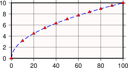
Linear transformation of Cartesian coordinates.
The complete commands given to produce this plot were
gmt psxy -R0/100/0/10 -JX3i/1.5i -Bag -BWSne+gsnow -Wthick,blue,- -P -K sqrt.d > GMT_linear.ps
gmt psxy -R -J -St0.1i -N -Gred -Wfaint -O sqrt.d10 >> GMT_linear.ps
Normally, the user’s x-values will increase to the right and the y-values will increase upwards. It should be noted that in many situations it is desirable to have the direction of positive coordinates be reversed. For example, when plotting depth on the y-axis it makes more sense to have the positive direction downwards. All that is required to reverse the sense of positive direction is to supply a negative scale (or axis length). Finally, sometimes it is convenient to specify the width (or height) of a map and let the other dimension be computed based on the implied scale and the range of the other axis. To do this, simply specify the length to be recomputed as 0.
13.1.1.2. Geographic coordinates
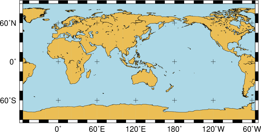
Linear transformation of map coordinates.
While the Cartesian linear projection is primarily designed for regular floating point x,y data, it is sometimes necessary to plot geographical data in a linear projection. This poses a problem since longitudes have a 360º periodicity. GMT therefore needs to be informed that it has been given geographical coordinates even though a linear transformation has been chosen. We do so by adding a g (for geographical) or d (for degrees) directly after -R or by appending a g or d to the end of the -Jx (or -JX) option. As an example, we want to plot a crude world map centered on 125ºE. Our command will be
gmt set MAP_GRID_CROSS_SIZE_PRIMARY 0.1i MAP_FRAME_TYPE FANCY FORMAT_GEO_MAP ddd:mm:ssF
gmt pscoast -Rg-55/305/-90/90 -Jx0.014i -Bagf -BWSen -Dc -A1000 -Glightbrown -Wthinnest \
        -P -Slightblue > GMT_linear_d.ps
with the result reproduced in Figure Linear transformation of map coordinates.
13.1.1.3. Calendar time coordinates
Linear transformation of calendar coordinates.
Several particular issues arise when we seek to make linear plots using calendar date/time as the input coordinates. As far as setting up the coordinate transformation we must indicate whether our input data have absolute time coordinates or relative time coordinates. For the former we append T after the axis scale (or width), while for the latter we append t at the end of the -Jx (or -JX) option. However, other command line arguments (like the -R option) may already specify whether the time coordinate is absolute or relative. An absolute time entry must be given as [date]T[clock] (with date given as yyyy[-mm[-dd]], yyyy[-jjj], or yyyy[-Www[-d]], and clock using the hh[:mm[:ss[.xxx]]] 24-hour clock format) whereas the relative time is simply given as the units of time since the epoch followed by t (see TIME_UNIT and TIME_EPOCH for information on specifying the time unit and the epoch). As a simple example, we will make a plot of a school week calendar (Figure Linear transformation of calendar coordinates).
When the coordinate ranges provided by the -R option and the projection type given by -JX (including the optional d, g, t or T) conflict, GMT will warn the users about it. In general, the options provided with -JX will prevail.
gmt set FORMAT_DATE_MAP o TIME_WEEK_START Sunday FORMAT_CLOCK_MAP=-hham \
        FORMAT_TIME_PRIMARY_MAP full
gmt psbasemap -R2001-9-24T/2001-9-29T/T07:0/T15:0 -JX4i/-2i -Bxa1Kf1kg1d \
              -Bya1Hg1h -BWsNe+glightyellow -P > GMT_linear_cal.ps
13.1.2. Cartesian logarithmic projection
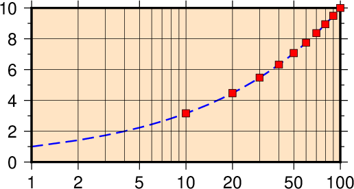
Logarithmic transformation of x--coordinates.
The \(\log_{10}\) transformation is simply \(u' = a \log_{10}(u) + b\) and is selected by appending an l (lower case L) immediately following the scale (or axis length) value. Hence, to produce a plot in which the x-axis is logarithmic (the y-axis remains linear, i.e., a semi-log plot), try (Figure Logarithmic transformation)
gmt psxy -R1/100/0/10 -Jx1.5il/0.15i -Bx2g3 -Bya2f1g2 -BWSne+gbisque \
         -Wthick,blue,- -P -K -h sqrt.d > GMT_log.ps
gmt psxy -R -J -Ss0.1i -N -Gred -W -O -h sqrt.d10 >> GMT_log.ps
Note that if x- and y-scaling are different and a \(\log_{10}-\log_{10}\) plot is desired, the l must be appended twice: Once after the x-scale (before the /) and once after the y-scale.
13.1.3. Cartesian power projection …
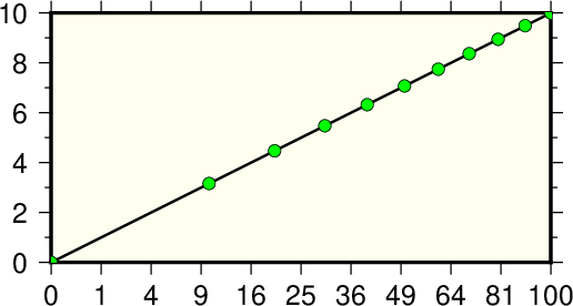
Exponential or power transformation of x--coordinates.
This projection uses \(u' = a u^b + c\) and allows us to explore exponential relationships like \(x^p\) versus \(y^q\). While p and q can be any values, we will select p = 0.5 and q = 1 which means we will plot x versus \(\sqrt{x}\). We indicate this scaling by appending a p (lower case P) followed by the desired exponent, in our case 0.5. Since q = 1 we do not need to specify p1 since it is identical to the linear transformation. Thus our command becomes (Figure Power transformation)
gmt psxy -R0/100/0/10 -Jx0.3ip0.5/0.15i -Bxa1p -Bya2f1 -BWSne+givory \
         -Wthick -P -K sqrt.d > GMT_pow.ps
gmt psxy -R -J -Sc0.075i -Ggreen -W -O sqrt.d10 >> GMT_pow.ps
13.2. Linear projection with polar coordinates (-Jp -JP) …
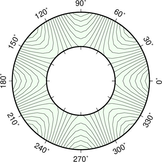
Polar (Cylindrical) transformation of (\(\theta, r\)) coordinates.
This transformation converts polar coordinates (angle \(\theta\) and radius r) to positions on a plot. Now \(x' = f(\theta,r)\) and \(y' = g(\theta,r)\), hence it is similar to a regular map projection because x and y are coupled and x (i.e., \(\theta\)) has a 360º periodicity. With input and output points both in the plane it is a two-dimensional projection. The transformation comes in two flavors:
- Normally, \(\theta\) is understood to be directions counter-clockwise from the horizontal axis, but we may choose to specify an angular offset [whose default value is zero]. We will call this offset \(\theta_0\). Then, \(x' = f(\theta, r) = ar \cos (\theta-\theta_0) + b\) and \(y' = g(\theta, r) = ar \sin (\theta-\theta_0) + c\).
- Alternatively, \(\theta\) can be interpreted to be azimuths clockwise from the vertical axis, yet we may again choose to specify the angular offset [whose default value is zero]. Then, \(x' = f(\theta, r) = ar \cos (90 - (\theta-\theta_0)) + b\) and \(y' = g(\theta, r) = ar \sin (90 - (\theta-\theta_0)) + c\).
Consequently, the polar transformation is defined by providing
- scale in inches/unit (-Jp) or full width of plot in inches (-JP)
- Optionally, insert a after p| P to indicate CW azimuths rather than CCW directions
- Optionally, append /origin in degrees to indicate an angular offset [0]
- Optionally, append r to reverse the radial direction (here, south and north must be elevations in 0--90 range).
- Optionally, append z to annotate depths rather than radius.
As an example of this projection we will create a gridded data set in polar coordinates \(z(\theta, r) = r^2 \cdot \cos{4\theta}\) using grdmath, a RPN calculator that operates on or creates grid files.
gmt grdmath -R0/360/2/4 -I6/0.1 X 4 MUL PI MUL 180 DIV COS Y 2 POW MUL = tt.nc
gmt grdcontour tt.nc -JP3i -B30 -BNs+ghoneydew -P -C2 -S4 --FORMAT_GEO_MAP=+ddd > GMT_polar.ps
We used grdcontour to make a contour map of this data. Because the data file only contains values with \(2 \leq r \leq 4\), a donut shaped plot appears in Figure Polar transformation.
14. GMT Map Projections
GMT implements more than 30 different projections. They all project the input coordinates longitude and latitude to positions on a map. In general, x’ = f(x,y,z) and y’ = g(x,y,z), where z is implicitly given as the radial vector length to the (x,y) point on the chosen ellipsoid. The functions f and g can be quite nasty and we will refrain from presenting details in this document. The interested read is referred to Snyder [1987] [20]. We will mostly be using the pscoast command to demonstrate each of the projections. GMT map projections are grouped into four categories depending on the nature of the projection. The groups are
- Conic map projections
- Azimuthal map projections
- Cylindrical map projections
- Miscellaneous projections
Because x and y are coupled we can only specify one plot-dimensional scale, typically a map scale (for lower-case map projection code) or a map width (for upper-case map projection code). However, in some cases it would be more practical to specify map height instead of width, while in other situations it would be nice to set either the shortest or longest map dimension. Users may select these alternatives by appending a character code to their map dimension. To specify map height, append h to the given dimension; to select the minimum map dimension, append -, whereas you may append + to select the maximum map dimension. Without the modifier the map width is selected by default.
In GMT version 4.3.0 we noticed we ran out of the alphabet for 1-letter (and sometimes 2-letter) projection codes. To allow more flexibility, and to make it easier to remember the codes, we implemented the option to use the abbreviations used by the Proj4 mapping package. Since some of the GMT projections are not in Proj4, we invented some of our own as well. For a full list of both the old 1- and 2-letter codes, as well as the Proj4-equivalents see the quick reference cards in Section GMT quick reference. For example, -JM15c and -JMerc/15c have the same meaning.
14.1. Conic projections
14.1.1. Albers conic equal-area projection (-Jb -JB) …
This projection, developed by Albers in 1805, is predominantly used to map regions of large east-west extent, in particular the United States. It is a conic, equal-area projection, in which parallels are unequally spaced arcs of concentric circles, more closely spaced at the north and south edges of the map. Meridians, on the other hand, are equally spaced radii about a common center, and cut the parallels at right angles. Distortion in scale and shape vanishes along the two standard parallels. Between them, the scale along parallels is too small; beyond them it is too large. The opposite is true for the scale along meridians. To define the projection in GMT you need to provide the following information:
- Longitude and latitude of the projection center.
- Two standard parallels.
- Map scale in inch/degree or 1:xxxxx notation (-Jb), or map width (-JB).
Note that you must include the “1:” if you choose to specify the scale that way. E.g., you can say 0.5 which means 0.5 inch/degree or 1:200000 which means 1 inch on the map equals 200,000 inches along the standard parallels. The projection center defines the origin of the rectangular map coordinates. As an example we will make a map of the region near Taiwan. We choose the center of the projection to be at 125ºE/20ºN and 25ºN and 45ºN as our two standard parallels. We desire a map that is 5 inches wide. The complete command needed to generate the map below is therefore given by:
gmt set MAP_GRID_CROSS_SIZE_PRIMARY 0
gmt pscoast -R110/140/20/35 -JB125/20/25/45/5i -Bag -Dl -Ggreen -Wthinnest \
            -A250 -P > GMT_albers.ps
Albers equal-area conic map projection.
14.1.2. Equidistant conic projection (-Jd -JD) …
The equidistant conic projection was described by the Greek philosopher Claudius Ptolemy about A.D. 150. It is neither conformal or equal-area, but serves as a compromise between them. The scale is true along all meridians and the standard parallels. To select this projection in GMT you must provide the same information as for the other conic projection, i.e.,
- Longitude and latitude of the projection center.
- Two standard parallels.
- Map scale in inch/degree or 1:xxxxx notation (-Jd), or map width (-JD).
The equidistant conic projection is often used for atlases with maps of small countries. As an example, we generate a map of Cuba:
gmt set FORMAT_GEO_MAP ddd:mm:ssF MAP_GRID_CROSS_SIZE_PRIMARY 0.05i
gmt pscoast -R-88/-70/18/24 -JD-79/21/19/23/4.5i -Bag -Di -N1/thick,red \
            -Glightgreen -Wthinnest -P > GMT_equidistant_conic.ps
Equidistant conic map projection.
14.1.3. Lambert conic conformal projection (-Jl -JL) …
This conic projection was designed by the Alsatian mathematician Johann Heinrich Lambert (1772) and has been used extensively for mapping of regions with predominantly east-west orientation, just like the Albers projection. Unlike the Albers projection, Lambert’s conformal projection is not equal-area. The parallels are arcs of circles with a common origin, and meridians are the equally spaced radii of these circles. As with Albers projection, it is only the two standard parallels that are distortion-free. To select this projection in GMT you must provide the same information as for the Albers projection, i.e.,
- Longitude and latitude of the projection center.
- Two standard parallels.
- Map scale in inch/degree or 1:xxxxx notation (-Jl), or map width (-JL).
The Lambert conformal projection has been used for basemaps for all the 48 contiguous States with the two fixed standard parallels 33ºN and 45ºN. We will generate a map of the continental USA using these parameters. Note that with all the projections you have the option of selecting a rectangular border rather than one defined by meridians and parallels. Here, we choose the regular WESN region, a “fancy” basemap frame, and use degrees west for longitudes. The generating commands used were
gmt set MAP_FRAME_TYPE FANCY FORMAT_GEO_MAP ddd:mm:ssF MAP_GRID_CROSS_SIZE_PRIMARY 0.05i
gmt pscoast -R-130/-70/24/52 -Jl-100/35/33/45/1:50000000 -Bag -Dl -N1/thick,red \
            -N2/thinner -A500 -Gtan -Wthinnest,white -Sblue -P > GMT_lambert_conic.ps
Lambert conformal conic map projection.
The choice for projection center does not affect the projection but it indicates which meridian (here 100ºW) will be vertical on the map. The standard parallels were originally selected by Adams to provide a maximum scale error between latitudes 30.5ºN and 47.5ºN of 0.5--1%. Some areas, like Florida, experience scale errors of up to 2.5%.
14.1.4. (American) polyconic projection (-Jpoly -JPoly) …
The polyconic projection, in Europe usually referred to as the American polyconic projection, was introduced shortly before 1820 by the Swiss-American cartographer Ferdinand Rodulph Hassler (1770--1843). As head of the Survey of the Coast, he was looking for a projection that would give the least distortion for mapping the coast of the United States. The projection acquired its name from the construction of each parallel, which is achieved by projecting the parallel onto the cone while it is rolled around the globe, along the central meridian, tangent to that parallel. As a consequence, the projection involves many cones rather than a single one used in regular conic projections.
The polyconic projection is neither equal-area, nor conformal. It is true to scale without distortion along the central meridian. Each parallel is true to scale as well, but the meridians are not as they get further away from the central meridian. As a consequence, no parallel is standard because conformity is lost with the lengthening of the meridians.
Below we reproduce the illustration by Snyder [1987], with a gridline every 10 and annotations only every 30º in longitude:
gmt pscoast -R-180/-20/0/90 -JPoly/4i -Bx30g10 -By10g10 -Dc -A1000 -Glightgray \
            -Wthinnest -P > GMT_polyconic.ps
(American) polyconic projection.
14.2. Azimuthal projections
14.2.1. Lambert Azimuthal Equal-Area (-Ja -JA)
This projection was developed by Lambert in 1772 and is typically used for mapping large regions like continents and hemispheres. It is an azimuthal, equal-area projection, but is not perspective. Distortion is zero at the center of the projection, and increases radially away from this point. To define this projection in GMT you must provide the following information:
- Longitude and latitude of the projection center.
- Optionally, the horizon, i.e., the number of degrees from the center to the edge (<= 180, default is 90).
- Scale as 1:xxxxx or as radius/latitude where radius is the projected distance on the map from projection center to an oblique latitude where 0 would be the oblique Equator (-Ja), or map width (-JA).
Two different types of maps can be made with this projection depending on how the region is specified. We will give examples of both types.
14.2.1.1. Rectangular map
In this mode we define our region by specifying the longitude/latitude of the lower left and upper right corners instead of the usual west, east, south, north boundaries. The reason for specifying our area this way is that for this and many other projections, lines of equal longitude and latitude are not straight lines and are thus poor choices for map boundaries. Instead we require that the map boundaries be rectangular by defining the corners of a rectangular map boundary. Using 0ºE/40ºS (lower left) and 60ºE/10ºS (upper right) as our corners we try
gmt set FORMAT_GEO_MAP ddd:mm:ssF MAP_GRID_CROSS_SIZE_PRIMARY 0
gmt pscoast -R0/-40/60/-10r -JA30/-30/4.5i -Bag -Dl -A500 -Gp300/10 \
            -Wthinnest -P > GMT_lambert_az_rect.ps
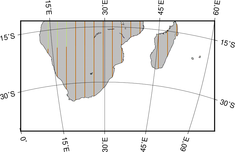
Rectangular map using the Lambert azimuthal equal-area projection.
Note that an “r” is appended to the -R option to inform GMT that the region has been selected using the rectangle technique, otherwise it would try to decode the values as west, east, south, north and report an error since ‘east’ < ‘west’.
14.2.1.2. Hemisphere map
Here, you must specify the world as your region (-Rg or -Rd). E.g., to obtain a hemisphere view that shows the Americas, try
gmt pscoast -Rg -JA280/30/3.5i -Bg -Dc -A1000 -Gnavy -P > GMT_lambert_az_hemi.ps
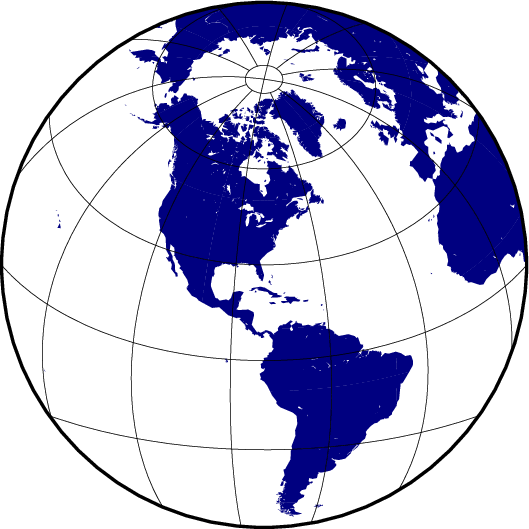
Hemisphere map using the Lambert azimuthal equal-area projection.
To geologists, the Lambert azimuthal equal-area projection (with origin at 0/0) is known as the equal-area (Schmidt) stereonet and used for plotting fold axes, fault planes, and the like. An equal-angle (Wulff) stereonet can be obtained by using the stereographic projection (discussed later). The stereonets produced by these two projections appear below.
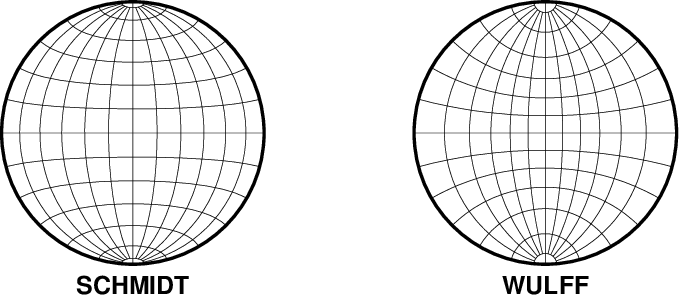
Equal-Area (Schmidt) and Equal-Angle (Wulff) stereo nets.
14.2.2. Stereographic Equal-Angle projection (-Js -JS) …
This is a conformal, azimuthal projection that dates back to the Greeks. Its main use is for mapping the polar regions. In the polar aspect all meridians are straight lines and parallels are arcs of circles. While this is the most common use it is possible to select any point as the center of projection. The requirements are
- Longitude and latitude of the projection center.
- Optionally, the horizon, i.e., the number of degrees from the center to the edge (< 180, default is 90).
- Scale as 1:xxxxx (true scale at pole), slat/1:xxxxx (true scale at standard parallel slat), or radius/latitude where radius is distance on map in inches from projection center to a particular oblique latitude (-Js), or simply map width (-JS).
A default map scale factor of 0.9996 will be applied by default (although you may change this with PROJ_SCALE_FACTOR). However, the setting is ignored when a standard parallel has been specified since the scale is then implicitly given. We will look at two different types of maps.
14.2.2.1. Polar Stereographic Map …
In our first example we will let the projection center be at the north pole. This means we have a polar stereographic projection and the map boundaries will coincide with lines of constant longitude and latitude. An example is given by
gmt pscoast -R-30/30/60/72 -Js0/90/4.5i/60 -B10g -Dl -A250 -Groyalblue \
            -Sseashell -P > GMT_stereographic_polar.ps
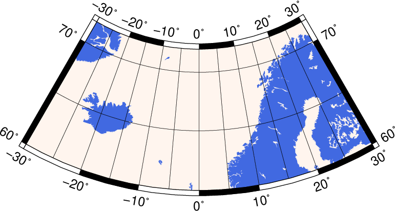
Polar stereographic conformal projection.
14.2.2.2. Rectangular stereographic map
As with Lambert’s azimuthal equal-area projection we have the option to use rectangular boundaries rather than the wedge-shape typically associated with polar projections. This choice is defined by selecting two points as corners in the rectangle and appending an “r” to the -R option. This command produces a map as presented in Figure Polar stereographic:
gmt set MAP_ANNOT_OBLIQUE 30
gmt pscoast -R-25/59/70/72r -JS10/90/11c -B20g -Dl -A250 -Gdarkbrown -Wthinnest \
            -Slightgray -P > GMT_stereographic_rect.ps
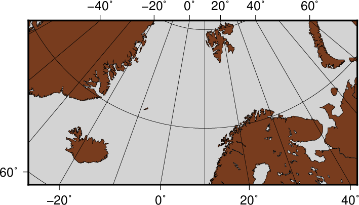
Polar stereographic conformal projection with rectangular borders.
14.2.2.3. General stereographic map
In terms of usage this projection is identical to the Lambert azimuthal equal-area projection. Thus, one can make both rectangular and hemispheric maps. Our example shows Australia using a projection pole at 130ºE/30ºS. The command used was
gmt set MAP_ANNOT_OBLIQUE 0
gmt pscoast -R100/-42/160/-8r -JS130/-30/4i -Bag -Dl -A500 -Ggreen -Slightblue \
            -Wthinnest -P > GMT_stereographic_general.ps
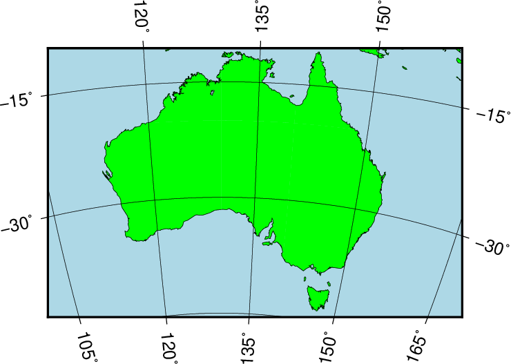
General stereographic conformal projection with rectangular borders.
By choosing 0/0 as the pole, we obtain the conformal stereonet presented next to its equal-area cousin in the Section Lambert Azimuthal Equal-Area (-Ja -JA) on the Lambert azimuthal equal-area projection (Figure Stereonets).
14.2.3. Perspective projection (-Jg -JG) …
The perspective projection imitates in 2 dimensions the 3-dimensional view of the earth from space. The implementation in GMT is very flexible, and thus requires many input variables. Those are listed and explained below, with the values used in Figure Perspective projection between brackets.
- Longitude and latitude of the projection center (4ºE/52ºN).
- Altitude of the viewer above sea level in kilometers (230 km). If this value is less than 10, it is assumed to be the distance of the viewer from the center of the earth in earth radii. If an “r” is appended, it is the distance from the center of the earth in kilometers.
- Azimuth in degrees (90, due east). This is the direction in which you are looking, measured clockwise from north.
- Tilt in degrees (60). This is the viewing angle relative to zenith. So a tilt of 0º is looking straight down, 60º is looking from 30º above the horizon.
- Twist in degrees (180). This is the boresight rotation (clockwise) of the image. The twist of 180º in the example mimics the fact that the Space Shuttle flies upside down.
- Width and height of the viewpoint in degrees (60). This number depends on whether you are looking with the naked eye (in which case you view is about 60º wide), or with binoculars, for example.
- Scale as 1:xxxxx or as radius/latitude where radius is distance on map in inches from projection center to a particular oblique latitude (-Jg), or map width (-JG) (5 inches).
The imagined view of northwest Europe from a Space Shuttle at 230 km looking due east is thus accomplished by the following pscoast command:
gmt pscoast -Rg -JG4/52/230/90/60/180/60/60/5i -Bx2g2 -By1g1 -Ia -Di -Glightbrown \
            -Wthinnest -P -Slightblue --MAP_ANNOT_MIN_SPACING=0.25i > GMT_perspective.ps
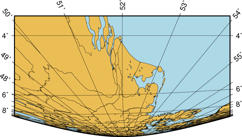
View from the Space Shuttle in Perspective projection.
14.2.4. Orthographic projection (-Jg -JG) …
The orthographic azimuthal projection is a perspective projection from infinite distance. It is therefore often used to give the appearance of a globe viewed from outer space. As with Lambert’s equal-area and the stereographic projection, only one hemisphere can be viewed at any time. The projection is neither equal-area nor conformal, and much distortion is introduced near the edge of the hemisphere. The directions from the center of projection are true. The projection was known to the Egyptians and Greeks more than 2,000 years ago. Because it is mainly used for pictorial views at a small scale, only the spherical form is necessary.
To specify the orthographic projection the same options -Jg or -JG as the perspective projection are used, but with fewer variables to supply:
- Longitude and latitude of the projection center.
- Optionally, the horizon, i.e., the number of degrees from the center to the edge (<= 90, default is 90).
- Scale as 1:xxxxx or as radius/latitude where radius is distance on map in inches from projection center to a particular oblique latitude (-Jg), or map width (-JG).
Our example of a perspective view centered on 75ºW/40ºN can therefore be generated by the following pscoast command:
gmt pscoast -Rg -JG-75/41/4.5i -Bg -Dc -A5000 -Gpink -Sthistle -P > GMT_orthographic.ps
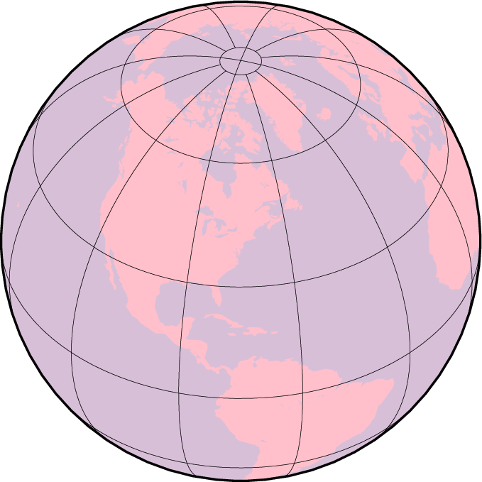
Hemisphere map using the Orthographic projection.
14.2.5. Azimuthal Equidistant projection (-Je -JE) …
The most noticeable feature of this azimuthal projection is the fact that distances measured from the center are true. Therefore, a circle about the projection center defines the locus of points that are equally far away from the plot origin. Furthermore, directions from the center are also true. The projection, in the polar aspect, is at least several centuries old. It is a useful projection for a global view of locations at various or identical distance from a given point (the map center).
To specify the azimuthal equidistant projection you must supply:
- Longitude and latitude of the projection center.
- Optionally, the horizon, i.e., the number of degrees from the center to the edge (<= 180, default is 180).
- Scale as 1:xxxxx or as radius/latitude where radius is distance on map in inches from projection center to a particular oblique latitude (-Je), or map width (-JE).
Our example of a global view centered on 100ºW/40ºN can therefore be generated by the following pscoast command. Note that the antipodal point is 180º away from the center, but in this projection this point plots as the entire map perimeter:
gmt pscoast -Rg -JE-100/40/4.5i -Bg -Dc -A10000 -Glightgray -Wthinnest -P \
            > GMT_az_equidistant.ps
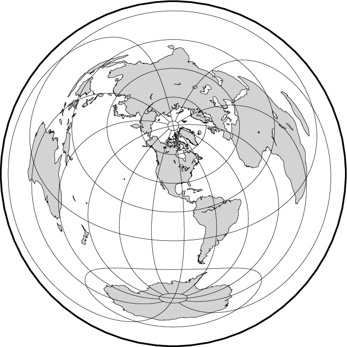
World map using the equidistant azimuthal projection.
14.2.6. Gnomonic projection (-Jf -JF) …
The Gnomonic azimuthal projection is a perspective projection from the center onto a plane tangent to the surface. Its origin goes back to the old Greeks who used it for star maps almost 2500 years ago. The projection is neither equal-area nor conformal, and much distortion is introduced near the edge of the hemisphere; in fact, less than a hemisphere may be shown around a given center. The directions from the center of projection are true. Great circles project onto straight lines. Because it is mainly used for pictorial views at a small scale, only the spherical form is necessary.
To specify the Gnomonic projection you must supply:
- Longitude and latitude of the projection center.
- Optionally, the horizon, i.e., the number of degrees from the center to the edge (< 90, default is 60).
- Scale as 1:xxxxx or as radius/latitude where radius is distance on map in inches from projection center to a particular oblique latitude (-Jf), or map width (-JF).
Using a horizon of 60, our example of this projection centered on 120ºW/35ºN can therefore be generated by the following pscoast command:
gmt pscoast -Rg -JF-120/35/60/4.5i -B30g15 -Dc -A10000 -Gtan -Scyan -Wthinnest \
            -P > GMT_gnomonic.ps
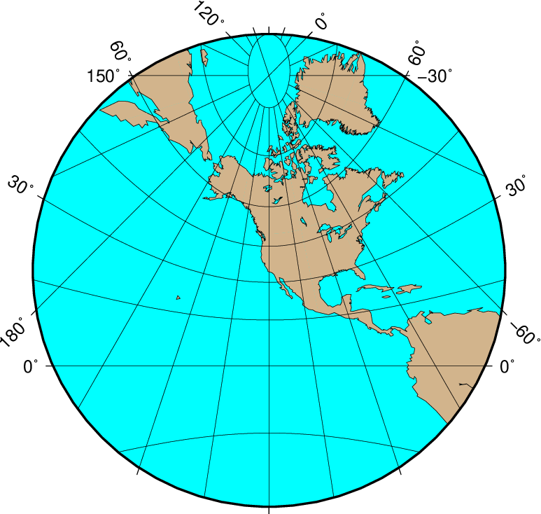
Gnomonic azimuthal projection.
14.3. Cylindrical projections
Cylindrical projections are easily recognized for its shape: maps are rectangular and meridians and parallels are straight lines crossing at right angles. But that is where similarities between the cylindrical projections supported by GMT (Mercator, transverse Mercator, universal transverse Mercator, oblique Mercator, Cassini, cylindrical equidistant, cylindrical equal-area, Miller, and cylindrical stereographic projections) stops. Each have a different way of spacing the meridians and parallels to obtain certain desirable cartographic properties.
14.3.1. Mercator projection (-Jm -JM) …
Probably the most famous of the various map projections, the Mercator projection takes its name from the Flemish cartographer Gheert Cremer, better known as Gerardus Mercator, who presented it in 1569. The projection is a cylindrical and conformal, with no distortion along the equator. A major navigational feature of the projection is that a line of constant azimuth is straight. Such a line is called a rhumb line or loxodrome. Thus, to sail from one point to another one only had to connect the points with a straight line, determine the azimuth of the line, and keep this constant course for the entire voyage [21]. The Mercator projection has been used extensively for world maps in which the distortion towards the polar regions grows rather large, thus incorrectly giving the impression that, for example, Greenland is larger than South America. In reality, the latter is about eight times the size of Greenland. Also, the Former Soviet Union looks much bigger than Africa or South America. One may wonder whether this illusion has had any influence on U.S. foreign policy.
In the regular Mercator projection, the cylinder touches the globe along the equator. Other orientations like vertical and oblique give rise to the Transverse and Oblique Mercator projections, respectively. We will discuss these generalizations following the regular Mercator projection.
The regular Mercator projection requires a minimum of parameters. To use it in GMT programs you supply this information (the first two items are optional and have defaults):
- Central meridian [Middle of your map].
- Standard parallel for true scale [Equator]. When supplied, central meridian must be supplied as well.
- Scale along the equator in inch/degree or 1:xxxxx (-Jm), or map width (-JM).
Our example presents a world map at a scale of 0.012 inch pr degree which will give a map 4.32 inch wide. It was created with the command:
gmt set MAP_FRAME_TYPE fancy
gmt pscoast -R0/360/-70/70 -Jm1.2e-2i -Bxa60f15 -Bya30f15 -Dc -A5000 -Gred \
            -P > GMT_mercator.ps
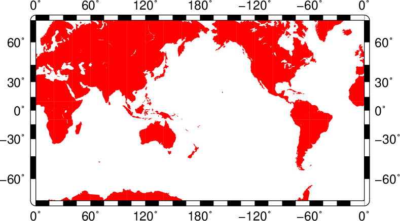
Simple Mercator map.
While this example is centered on the Dateline, one can easily choose another configuration with the -R option. A map centered on Greenwich would specify the region with -R-180/180/-70/70.
14.3.2. Transverse Mercator projection (-Jt -JT) …
The transverse Mercator was invented by Lambert in 1772. In this projection the cylinder touches a meridian along which there is no distortion. The distortion increases away from the central meridian and goes to infinity at 90º from center. The central meridian, each meridian 90º away from the center, and equator are straight lines; other parallels and meridians are complex curves. The projection is defined by specifying:
- The central meridian.
- Optionally, the latitude of origin (default is the equator).
- Scale along the equator in inch/degree or 1:xxxxx (-Jt), or map width (-JT).
The optional latitude of origin defaults to Equator if not specified. Although defaulting to 1, you can change the map scale factor via the PROJ_SCALE_FACTOR parameter. Our example shows a transverse Mercator map of south-east Europe and the Middle East with 35ºE as the central meridian:
gmt pscoast -R20/30/50/45r -Jt35/0.18i -Bag -Dl -A250 -Glightbrown -Wthinnest \
            -P -Sseashell > GMT_transverse_merc.ps
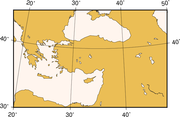
Rectangular Transverse Mercator map.
The transverse Mercator can also be used to generate a global map - the equivalent of the 360º Mercator map. Using the command
gmt pscoast -R0/360/-80/80 -JT330/-45/3.5i -Ba30g -BWSne -Dc -A2000 \
            -Slightblue -G0 -P > GMT_TM.ps
we made the map illustrated in Figure Global transverse Mercator. Note that when a world map is given (indicated by -R0/360/s/n), the arguments are interpreted to mean oblique degrees, i.e., the 360º range is understood to mean the extent of the plot along the central meridian, while the “south” and “north” values represent how far from the central longitude we want the plot to extend. These values correspond to latitudes in the regular Mercator projection and must therefore be less than 90.
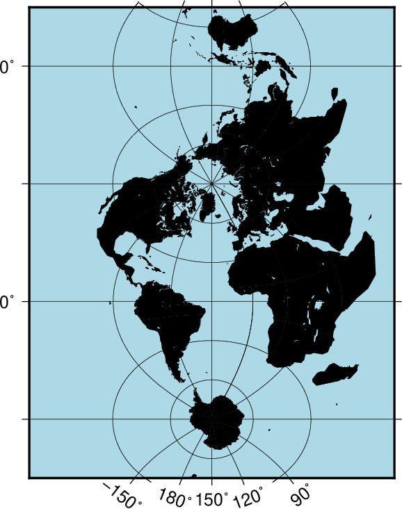
A global transverse Mercator map.
14.3.3. Universal Transverse Mercator (UTM) projection (-Ju -JU) …
A particular subset of the transverse Mercator is the Universal Transverse Mercator (UTM) which was adopted by the US Army for large-scale military maps. Here, the globe is divided into 60 zones between 84ºS and 84ºN, most of which are 6 wide. Each of these UTM zones have their unique central meridian. Furthermore, each zone is divided into latitude bands but these are not needed to specify the projection for most cases. See Figure Universal Transverse Mercator for all zone designations.
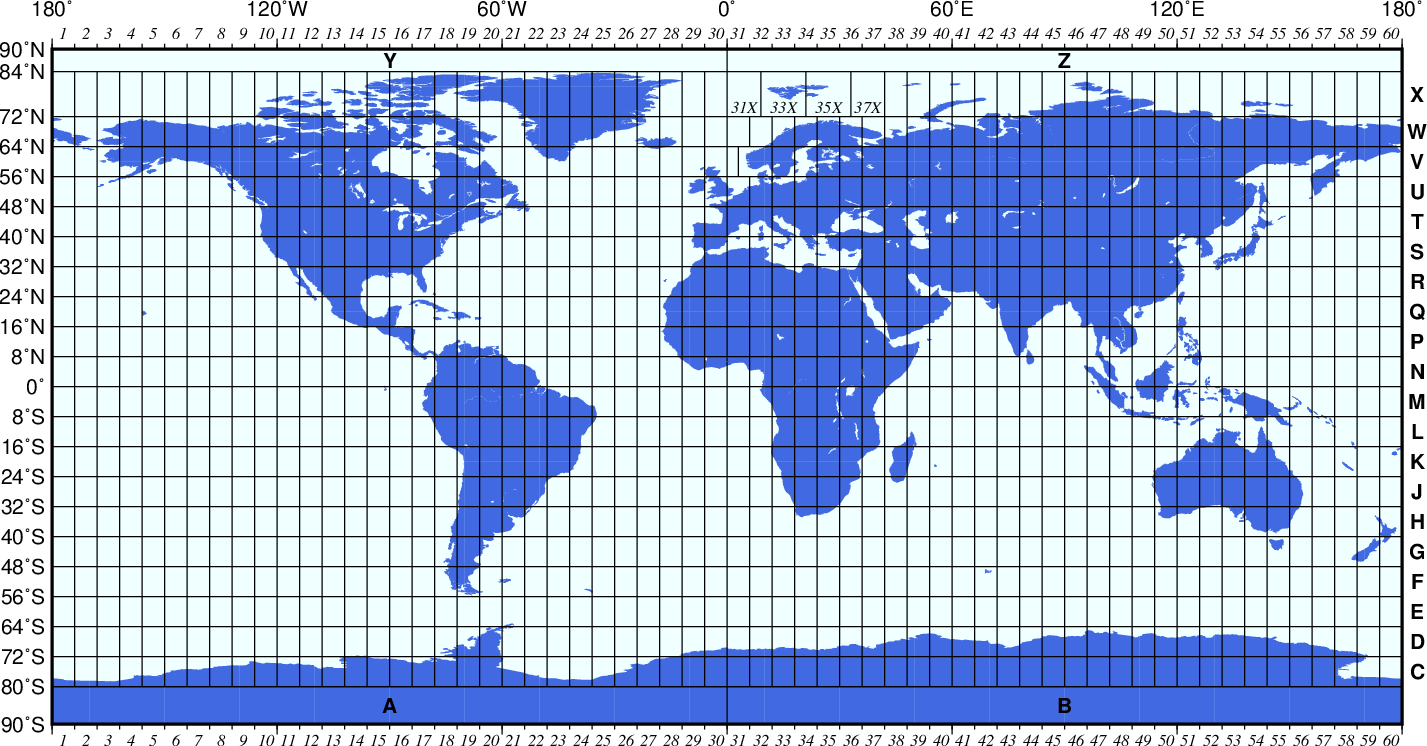
Universal Transverse Mercator zone layout.
GMT implements both the transverse Mercator and the UTM projection. When selecting UTM you must specify:
- UTM zone (A, B, 1--60, Y, Z). Use negative values for numerical zones in the southern hemisphere or append the latitude modifiers C--H, J--N, P--X) to specify an exact UTM grid zone.
- Scale along the equator in inch/degree or 1:xxxxx (-Ju), or map width (-JU).
In order to minimize the distortion in any given zone, a scale factor of 0.9996 has been factored into the formulae. (although a standard, you can change this with PROJ_SCALE_FACTOR). This makes the UTM projection a secant projection and not a tangent projection like the transverse Mercator above. The scale only varies by 1 part in 1,000 from true scale at equator. The ellipsoidal projection expressions are accurate for map areas that extend less than 10 away from the central meridian. For larger regions we use the conformal latitude in the general spherical formulae instead.
14.3.4. Oblique Mercator projection (-Jo -JO) …
Oblique configurations of the cylinder give rise to the oblique Mercator projection. It is particularly useful when mapping regions of large lateral extent in an oblique direction. Both parallels and meridians are complex curves. The projection was developed in the early 1900s by several workers. Several parameters must be provided to define the projection. GMT offers three different definitions:
- Option -Jo[a|A] or -JO[a|A]:
- Longitude and latitude of projection center.
- Azimuth of the oblique equator.
- Scale in inch/degree or 1:xxxxx along oblique equator (-Jo), or map width (-JO).
- Option -Jo[b|B] or -JO[b|B]:
- Longitude and latitude of projection center.
- Longitude and latitude of second point on oblique equator.
- Scale in inch/degree or 1:xxxxx along oblique equator (-Jo), or map width (-JO).
- Option -Joc|C or -JOc|C:
- Longitude and latitude of projection center.
- Longitude and latitude of projection pole.
- Scale in inch/degree or 1:xxxxx along oblique equator (-Jo), or map width (-JO).
For all three definitions, the upper case A|B|C means we will allow projection poles in the southern hemisphere [By default we map any such poles to their antipodes in the north hemisphere]. Our example was produced by the command
gmt pscoast -R270/20/305/25r -JOc280/25.5/22/69/4.8i -Bag -Di -A250 -Gburlywood \
            -Wthinnest -P -TdjTR+w0.4i+f2+l+o0.15i -Sazure --FONT_TITLE=8p \
            --MAP_TITLE_OFFSET=0.05i > GMT_obl_merc.ps
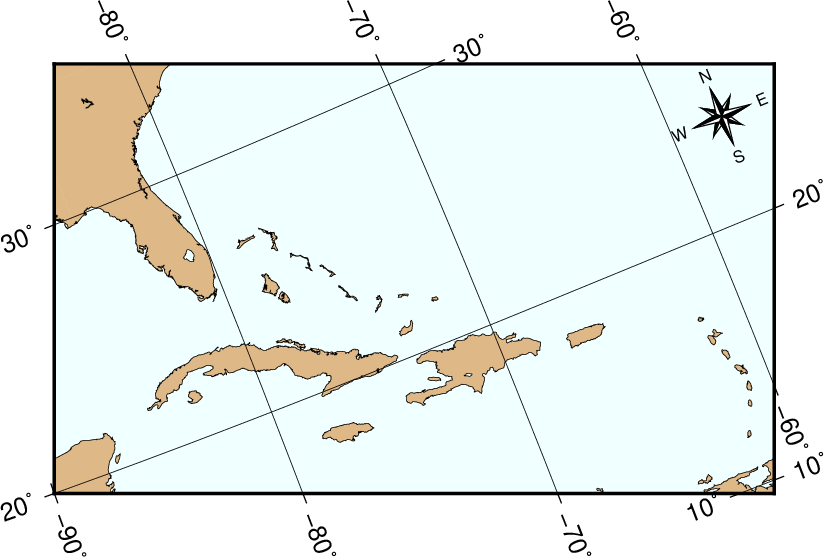
Oblique Mercator map using -Joc. We make it clear which direction is North by adding a star rose with the -Td option.
It uses definition 3 for an oblique view of some Caribbean islands. Note that we define our region using the rectangular system described earlier. If we do not append an “r” to the -R string then the information provided with the -R option is assumed to be oblique degrees about the projection center rather than the usual geographic coordinates. This interpretation is chosen since in general the parallels and meridians are not very suitable as map boundaries.
When working with oblique projections such as here, it is often much more convenient to specify the map domain in the projected coordinates relative to the map center. The figure below shows two views of New Zealand using the oblique Mercator projection that in both cases specifies the region using -Rk-1000/1000/-500/500. The leading unit k means the following bounds are in projected km and we let GMT determine the geographic coordinates of the two diagonal corners internally.
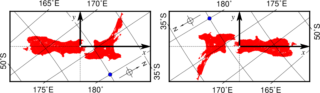
(left) Oblique view of New Zealand centered on its geographical center (Nelson) indicated by the white circle for an oblique Equator with azimuth 35. This resulted in the argument -JOa173:17:02E/41:16:15S/35/3i. The map is 2000 km by 1000 km and the Cartesian coordinate system in the projected units are indicated by the bold axes. The blue circle is the point (40S,180E) and it has projected coordinates (x = 426.2, y = -399.7). (right) Same dimensions but now specifying an azimuth of 215, yielding a projection pole in the southern hemisphere (hence we used -JOA to override the restriction, i.e., -JOA173:17:02E/41:16:15S/215/3i.) The projected coordinate system is still aligned as before but the Earth has been rotated 180 degrees. The blue point now has projected coordinates (x = -426.2, y = 399.7).
14.3.5. Cassini cylindrical projection (-Jc -JC) …
This cylindrical projection was developed in 1745 by César-François Cassini de Thury for the survey of France. It is occasionally called Cassini-Soldner since the latter provided the more accurate mathematical analysis that led to the development of the ellipsoidal formulae. The projection is neither conformal nor equal-area, and behaves as a compromise between the two end-members. The distortion is zero along the central meridian. It is best suited for mapping regions of north-south extent. The central meridian, each meridian 90º away, and equator are straight lines; all other meridians and parallels are complex curves. The requirements to define this projection are:
- Longitude and latitude of central point.
- Scale in inch/degree or as 1:xxxxx (-Jc), or map width (-JC).
A detailed map of the island of Sardinia centered on the 8º45’E meridian using the Cassini projection can be obtained by running the command:
gmt pscoast -R7:30/38:30/10:30/41:30r -JC8.75/40/2.5i -Bafg -LjBR+c40+w100+f+o0.15i/0.2i -Gspringgreen \
            -Dh -Sazure -Wthinnest -Ia/thinner -P --FONT_LABEL=12p > GMT_cassini.ps
Cassini map over Sardinia.
As with the previous projections, the user can choose between a rectangular boundary (used here) or a geographical (WESN) boundary.
14.3.6. Cylindrical equidistant projection (-Jq -JQ) …
This simple cylindrical projection is really a linear scaling of longitudes and latitudes. The most common form is the Plate Carrée projection, where the scaling of longitudes and latitudes is the same. All meridians and parallels are straight lines. The projection can be defined by:
- The central meridian [Middle of your map].
- Standard parallel [Equator].
- Scale in inch/degree or as 1:xxxxx (-Jq), or map width (-JQ).
The first two of these are optional and have defaults. When the standard parallel is defined, the central meridian must be supplied as well.
A world map centered on the dateline using this projection can be obtained by running the command:
gmt pscoast -Rg -JQ4.5i -B60f30g30 -Dc -A5000 -Gtan4 -Slightcyan -P > GMT_equi_cyl.ps
World map using the Plate Carrée projection.
Different relative scalings of longitudes and latitudes can be obtained by selecting a standard parallel different from the equator. Some selections for standard parallels have practical properties as shown in Table JQ.
| Grafarend and Niermann, minimum linear distortion | 61.7º |
| Ronald Miller Equirectangular | 50.5º |
| Ronald Miller, minimum continental distortion | 43.5º |
| Grafarend and Niermann | 42º |
| Ronald Miller, minimum overall distortion | 37.5º |
| Plate Carrée, Simple Cylindrical, Plain/Plane | 0º |
14.3.7. Cylindrical equal-area projections (-Jy -JY) …
This cylindrical projection is actually several projections, depending on what latitude is selected as the standard parallel. However, they are all equal area and hence non-conformal. All meridians and parallels are straight lines. The requirements to define this projection are:
- The central meridian.
- The standard parallel.
- Scale in inch/degree or as 1:xxxxx (-Jy), or map width (-JY)
While you may choose any value for the standard parallel and obtain your own personal projection, there are seven choices of standard parallels that result in known (or named) projections. These are listed in Table JY.
| Balthasart | 50º |
| Gall | 45º |
| Hobo-Dyer | 37º30’ (= 37.5º) |
| Trystan Edwards | 37º24’ (= 37.4º) |
| Caster | 37º04’ (= 37.0666º) |
| Behrman | 30º |
| Lambert | 0º |
For instance, a world map centered on the 35ºE meridian using the Behrman projection (Figure Behrman cylindrical projection) can be obtained by running the command:
gmt pscoast -R-145/215/-90/90 -JY35/30/4.5i -B45g45 -Dc -A10000 -Sdodgerblue \
            -Wthinnest -P > GMT_general_cyl.ps
World map using the Behrman cylindrical equal-area projection.
As one can see there is considerable distortion at high latitudes since the poles map into lines.
14.3.8. Miller Cylindrical projection (-Jj -JJ) …
This cylindrical projection, presented by Osborn Maitland Miller of the American Geographic Society in 1942, is neither equal nor conformal. All meridians and parallels are straight lines. The projection was designed to be a compromise between Mercator and other cylindrical projections. Specifically, Miller spaced the parallels by using Mercator’s formula with 0.8 times the actual latitude, thus avoiding the singular poles; the result was then divided by 0.8. There is only a spherical form for this projection. Specify the projection by:
- Optionally, the central meridian (default is the middle of your map).
- Scale in inch/degree or as 1:xxxxx (-Jj), or map width (-JJ).
For instance, a world map centered on the 90ºE meridian at a map scale of 1:400,000,000 (Figure Miller projection) can be obtained as follows:
gmt pscoast -R-90/270/-80/90 -Jj1:400000000 -Bx45g45 -By30g30 -Dc -A10000 \
            -Gkhaki -Wthinnest -P -Sazure > GMT_miller.ps
World map using the Miller cylindrical projection.
14.3.9. Cylindrical stereographic projections (-Jcyl_stere -JCyl_stere) …
The cylindrical stereographic projections are certainly not as notable as other cylindrical projections, but are still used because of their relative simplicity and their ability to overcome some of the downsides of other cylindrical projections, like extreme distortions of the higher latitudes. The stereographic projections are perspective projections, projecting the sphere onto a cylinder in the direction of the antipodal point on the equator. The cylinder crosses the sphere at two standard parallels, equidistant from the equator. The projections are defined by:
- The central meridian (uses the middle of the map when omitted).
- The standard parallel (default is the Equator). When used, central meridian needs to be given as well.
- Scale in inch/degree or as 1:xxxxx (-Jcyl_stere), or map width (-JCyl_stere)
Some of the selections of the standard parallel are named for the cartographer or publication that popularized the projection (Table JCylstere).
| Miller’s modified Gall | 66.159467º |
| Kamenetskiy’s First | 55º |
| Gall’s stereographic | 45º |
| Bolshoi Sovietskii Atlas Mira or Kamenetskiy’s Second | 30º |
| Braun’s cylindrical | 0º |
A map of the world, centered on the Greenwich meridian, using the Gall’s stereographic projection (standard parallel is 45º, Figure Gall’s stereographic projection), is obtained as follows:
gmt set FORMAT_GEO_MAP dddA
gmt pscoast -R-180/180/-60/80 -JCyl_stere/0/45/4.5i -Bxa60f30g30 -Bya30g30 -Dc -A5000 \
            -Wblack -Gseashell4 -Santiquewhite1 -P > GMT_gall_stereo.ps
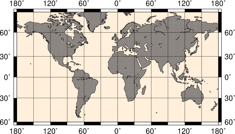
World map using Gall’s stereographic projection.
14.4. Miscellaneous projections
GMT supports 8 common projections for global presentation of data or models. These are the Hammer, Mollweide, Winkel Tripel, Robinson, Eckert IV and VI, Sinusoidal, and Van der Grinten projections. Due to the small scale used for global maps these projections all use the spherical approximation rather than more elaborate elliptical formulae.
In all cases, the specification of the central meridian can be skipped. The default is the middle of the longitude range of the plot, specified by the (-R) option.
14.4.1. Hammer projection (-Jh -JH) …
The equal-area Hammer projection, first presented by the German mathematician Ernst von Hammer in 1892, is also known as Hammer-Aitoff (the Aitoff projection looks similar, but is not equal-area). The border is an ellipse, equator and central meridian are straight lines, while other parallels and meridians are complex curves. The projection is defined by selecting:
- The central meridian [Middle of your map].
- Scale along equator in inch/degree or 1:xxxxx (-Jh), or map width (-JH).
A view of the Pacific ocean using the Dateline as central meridian is accomplished thus
gmt pscoast -Rg -JH4.5i -Bg -Dc -A10000 -Gblack -Scornsilk -P > GMT_hammer.ps
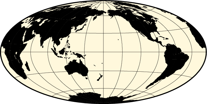
World map using the Hammer projection.
14.4.2. Mollweide projection (-Jw -JW) …
This pseudo-cylindrical, equal-area projection was developed by the German mathematician and astronomer Karl Brandan Mollweide in 1805. Parallels are unequally spaced straight lines with the meridians being equally spaced elliptical arcs. The scale is only true along latitudes 4044’ north and south. The projection is used mainly for global maps showing data distributions. It is occasionally referenced under the name homalographic projection. Like the Hammer projection, outlined above, we need to specify only two parameters to completely define the mapping of longitudes and latitudes into rectangular x/y coordinates:
- The central meridian [Middle of your map].
- Scale along equator in inch/degree or 1:xxxxx (-Jw), or map width (-JW).
An example centered on Greenwich can be generated thus:
gmt pscoast -Rd -JW4.5i -Bg -Dc -A10000 -Gtomato1 -Sskyblue -P > GMT_mollweide.ps
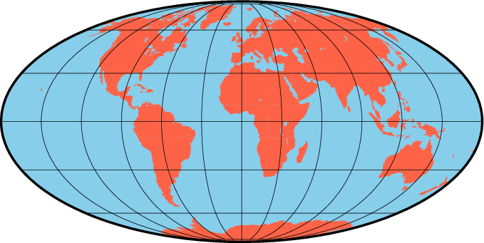
World map using the Mollweide projection.
14.4.3. Winkel Tripel projection (-Jr -JR) …
In 1921, the German mathematician Oswald Winkel a projection that was to strike a compromise between the properties of three elements (area, angle and distance). The German word “tripel” refers to this junction of where each of these elements are least distorted when plotting global maps. The projection was popularized when Bartholomew and Son started to use it in its world-renowned “The Times Atlas of the World” in the mid 20th century. In 1998, the National Geographic Society made the Winkel Tripel as its map projection of choice for global maps.
Naturally, this projection is neither conformal, nor equal-area. Central meridian and equator are straight lines; other parallels and meridians are curved. The projection is obtained by averaging the coordinates of the Equidistant Cylindrical and Aitoff (not Hammer-Aitoff) projections. The poles map into straight lines 0.4 times the length of equator. To use it you must enter
- The central meridian [Middle of your map].
- Scale along equator in inch/degree or 1:xxxxx (-Jr), or map width (-JR).
Centered on Greenwich, the example in Figure Winkel Tripel projection was created by this command:
gmt pscoast -Rd -JR4.5i -Bg -Dc -A10000 -Gburlywood4 -Swheat1 -P > GMT_winkel.ps
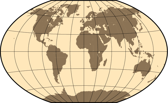
World map using the Winkel Tripel projection.
14.4.4. Robinson projection (-Jn -JN) …
The Robinson projection, presented by the American geographer and cartographer Arthur H. Robinson in 1963, is a modified cylindrical projection that is neither conformal nor equal-area. Central meridian and all parallels are straight lines; other meridians are curved. It uses lookup tables rather than analytic expressions to make the world map “look” right [22]. The scale is true along latitudes 38. The projection was originally developed for use by Rand McNally and is currently used by the National Geographic Society. To use it you must enter
- The central meridian [Middle of your map].
- Scale along equator in inch/degree or 1:xxxxx (-Jn), or map width (-JN).
Again centered on Greenwich, the example below was created by this command:
gmt pscoast -Rd -JN4.5i -Bg -Dc -A10000 -Ggoldenrod -Ssnow2 -P > GMT_robinson.ps
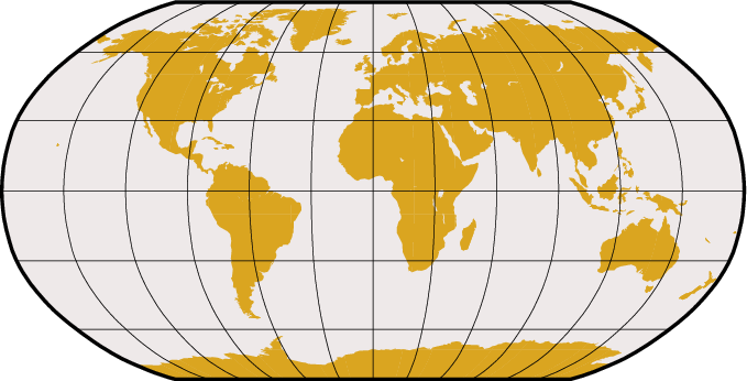
World map using the Robinson projection.
14.4.5. Eckert IV and VI projection (-Jk -JK) …
The Eckert IV and VI projections, presented by the German cartographer Max Eckert-Greiffendorff in 1906, are pseudo-cylindrical equal-area projections. Central meridian and all parallels are straight lines; other meridians are equally spaced elliptical arcs (IV) or sinusoids (VI). The scale is true along latitudes 40º30’ (IV) and 49º16’ (VI). Their main use is in thematic world maps. To select Eckert IV you must use -JKf (f for “four”) while Eckert VI is selected with -JKs (s for “six”). If no modifier is given it defaults to Eckert VI. In addition, you must enter
- The central meridian [Middle of your map].
- Scale along equator in inch/degree or 1:xxxxx (-Jk), or map width (-JK).
Centered on the Dateline, the Eckert IV example below was created by this command:
gmt pscoast -Rg -JKf4.5i -Bg -Dc -A10000 -Wthinnest -Givory -Sbisque3 -P > GMT_eckert4.ps
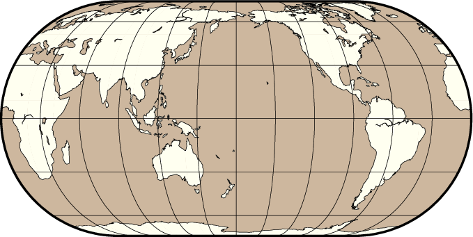
World map using the Eckert IV projection.
The same script, with s instead of f, yields the Eckert VI map:
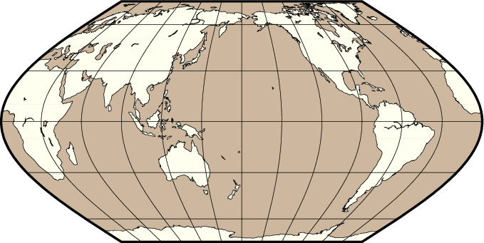
World map using the Eckert VI projection.
14.4.6. Sinusoidal projection (-Ji -JI) …
The sinusoidal projection is one of the oldest known projections, is equal-area, and has been used since the mid-16th century. It has also been called the “Equal-area Mercator” projection. The central meridian is a straight line; all other meridians are sinusoidal curves. Parallels are all equally spaced straight lines, with scale being true along all parallels (and central meridian). To use it, you need to select:
- The central meridian [Middle of your map].
- Scale along equator in inch/degree or 1:xxxxx (-Ji), or map width (-JI).
A simple world map using the sinusoidal projection is therefore obtained by
gmt pscoast -Rd -JI4.5i -Bxg30 -Byg15 -Dc -A10000 -Ggray -P > GMT_sinusoidal.ps
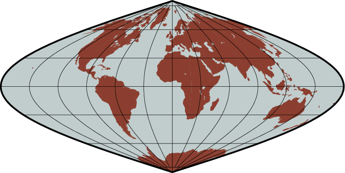
World map using the Sinusoidal projection.
To reduce distortion of shape the interrupted sinusoidal projection was introduced in 1927. Here, three symmetrical segments are used to cover the entire world. Traditionally, the interruptions are at 160ºW, 20ºW, and 60ºE. To make the interrupted map we must call pscoast for each segment and superpose the results. To produce an interrupted world map (with the traditional boundaries just mentioned) that is 5.04 inches wide we use the scale 5.04/360 = 0.014 and offset the subsequent plots horizontally by their widths (140\(\cdot\)0.014 and 80\(\cdot\)0.014):
gmt pscoast -R200/340/-90/90 -Ji0.014i -Bxg30 -Byg15 -A10000 -Dc \
            -Gblack -K -P > GMT_sinus_int.ps
gmt pscoast -R-20/60/-90/90 -Ji0.014i -Bxg30 -Byg15 -Dc -A10000 \
            -Gblack -X1.96i -O -K >> GMT_sinus_int.ps
gmt pscoast -R60/200/-90/90 -Ji0.014i -Bxg30 -Byg15 -Dc -A10000 \
            -Gblack -X1.12i -O >> GMT_sinus_int.ps
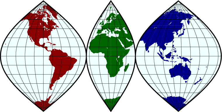
World map using the Interrupted Sinusoidal projection.
The usefulness of the interrupted sinusoidal projection is basically limited to display of global, discontinuous data distributions like hydrocarbon and mineral resources, etc.
14.4.7. Van der Grinten projection (-Jv -JV) …
The Van der Grinten projection, presented by Alphons J. van der Grinten in 1904, is neither equal-area nor conformal. Central meridian and Equator are straight lines; other meridians are arcs of circles. The scale is true along the Equator only. Its main use is to show the entire world enclosed in a circle. To use it you must enter
- The central meridian [Middle of your map].
- Scale along equator in inch/degree or 1:xxxxx (-Jv), or map width (-JV).
Centered on the Dateline, the example below was created by this command:
gmt pscoast -Rg -JV4i -Bxg30 -Byg15 -Dc -Glightgray -A10000 \
            -Wthinnest -P > GMT_grinten.ps
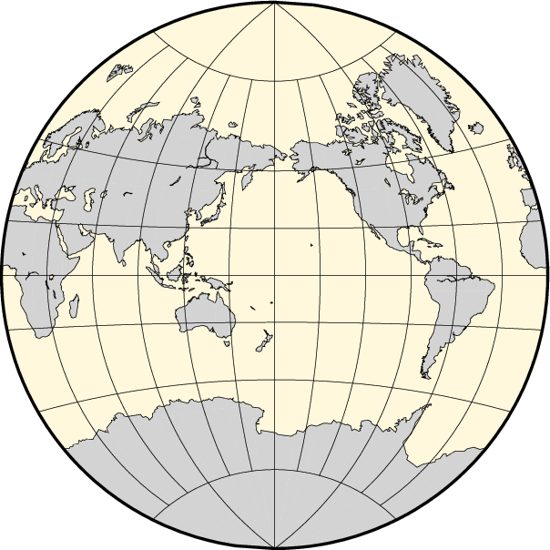
World map using the Van der Grinten projection.
17. GMT Supplemental Packages
These packages are for the most part written and supported by us, but
there are some exceptions. They provide extensions of GMT that are
needed for particular rather than general applications.
Questions or bug reports for this software
should be addressed to the person(s) listed in the README file associated with
the particular program. It is not guaranteed that these programs are
fully ANSI-C, Y2K, or POSIX compliant, or that they necessarily will
install smoothly on all platforms, but most do. Note that the data sets
some of these programs work on are not distributed with these packages;
they must be obtained separately. The contents of the supplemental
archive may change without notice; at this writing it contains these directories:
17.1. gshhg: GSHHG data extractor
This package contains gshhg which you can use to extract shoreline polygons from the Global Self-consistent Hierarchical High-resolution Shorelines (GSHHG) available separately from or the (GSHHG is the polygon data base from which the GMT coastlines derive). The package is maintained by Paul Wessel.
17.2. img: gridded altimetry extractor
This package consists of the program img2grd to extract subsets of the global gravity and predicted topography solutions derived from satellite altimetry [28]. The package is maintained by Walter Smith and Paul Wessel.
17.3. meca: seismology and geodesy symbols
This package contains the programs pscoupe, psmeca, pspolar, psvelo, and pssac which are used by seismologists and geodesists for plotting focal mechanisms (including cross-sections and polarities), error ellipses, velocity arrows, rotational wedges, and more. The package was developed by Kurt Feigl and Genevieve Patau with contributions from Dongdong Tian but is now maintained by the GMT team.
17.4. mgd77: MGD77 extractor and plotting tools
This package currently holds the programs mgd77convert, mgd77header, mgd77info, mgd77list, mgd77magref, mgd77manage, mgd77path, mgd77sniffer, and mgd77track which can be used to extract information or data values from or plot marine geophysical data files in the ASCII MGD77 or netCDF MGD77+ formats [29]). This package has replaced the old mgg package. The package is maintained by Paul Wessel and Mike Chandler.
17.5. misc: Miscellaneous tools
At the moment, this package contains the program dimfilter, which is an extension of grdfilter in that it allows for spatial directional filtering. The package is maintained by Paul Wessel.
17.6. potential: Geopotential tools
At the moment, this package contains the programs gravfft, which performs gravity, isostasy, and admittance calculation for grids, grdredpol, which compute the continuous reduction to the pole, AKA differential RTP for magnetic data, grdseamount, which computes synthetic bathymetry over various seamount shapes, and gmtgravmag3d and grdgravmag3d, which computes the gravity or magnetic anomaly of a body by the method of Okabe [30], and talwani2d and talwani3d and which uses the methods of Talwani to compute various geopotential components from 2-D [31] or 3-D [32] bodies. The package is maintained by Joaquim Luis and Paul Wessel.
17.7. segyprogs: plotting SEGY seismic data
This package contains programs to plot SEGY seismic data files using the GMT mapping transformations and postscript library. pssegy generates a 2-D plot (x:location and y:time/depth) while pssegyz generates a 3-D plot (x and y: location coordinates, z: time/depth). Locations may be read from predefined or arbitrary portions of each trace header. Finally, segy2grd can convert SEGY data to a GMT grid file. The package is maintained by Tim Henstock [33].
17.8. spotter: backtracking and hotspotting
This package contains the plate tectonic programs backtracker, which you can use to move geologic markers forward or backward in time, grdpmodeler which evaluates predictions of a plate motion model on a grid, grdrotater which rotates entire grids using a finite rotation, hotspotter which generates CVA grids based on seamount locations and a set of absolute plate motion stage poles (grdspotter does the same using a bathymetry grid instead of seamount locations), originator, which associates seamounts with the most likely hotspot origins, and rotconverter which does various operations involving finite rotations on a sphere. The package is maintained by Paul Wessel.
17.9. x2sys: track crossover error estimation
This package contains the tools x2sys_datalist, which allows you to extract data from almost any binary or ASCII data file, and x2sys_cross which determines crossover locations and errors generated by one or several geospatial tracks. Newly added are the tools x2sys_init, x2sys_binlist, x2sys_get, x2sys_list, x2sys_put, x2sys_report, x2sys_solve and x2sys_merge which extends the track-management system employed by the mgg supplement to generic track data of any format. This package represents a new generation of tools and replaces the old x_system package. The package is maintained by Paul Wessel.
18. GMT File Formats
18.1. Table data
These files have N records which have M fields each. All programs that handle tables can read multicolumn files. GMT can read both ASCII, native binary, and netCDF table data. For other formats (e.g., ESRI shapefiles), convert them to GMT/OGR format via GDAL’s ogr2ogr tool first.
18.1.1. ASCII tables
18.1.1.1. Optional file header records
The first data record may be preceded by one or more header records. Any records that begins with ‘#’ is considered a header or comment line and are always processed correctly. If your data file has leading header records that do not start with ‘#’ then you must make sure to use the -h option and set the parameter IO_N_HEADER_RECS in the gmt.conf file (GMT default is one header record if -h is given; you may also use -hnrecs directly). Fields within a record must be separated by spaces, tabs, commas, or semi-colons. Each field can be an integer or floating-point number or a geographic coordinate string using the [±]dd[:mm[:ss]][W:|S|N|E|w|s|n|e] format. Thus, 12:30:44.5W, 17.5S, 1:00:05, and 200:45E are all valid input strings. GMT is expected to handle most CVS (Comma-Separated Values) files, including numbers given in double quotes. On output, fields will be separated by the character given by the parameter IO_COL_SEPARATOR, which by default is a TAB.
18.1.1.2. Optional segment header records
When dealing with time- or (x,y)-series it is usually convenient to have each profile in separate files. However, this may sometimes prove impractical due to large numbers of profiles. An example is files of digitized lineations where the number of individual features may range into the thousands. One file per feature would in this case be unreasonable and furthermore clog up the directory. GMT provides a mechanism for keeping more than one profile in a file. Such files are called multiple segment files and are identical to the ones just outlined except that they have segment headers interspersed with data records that signal the start of a new segment. The segment headers may be of any format, but all must have the same character in the first column. The unique character is by default ‘>’, but you can override that by modifying the IO_SEGMENT_MARKER default setting. Programs can examine the segment headers to see if they contain -D for a distance value, -W and -G options for specifying pen and fill attributes for individual segments, -Z to change color via a CPT, -L for label specifications, or -T for general-purpose text descriptions. These settings (and occasionally others) will override the corresponding command line options. GMT also provides for two special values for IO_SEGMENT_MARKER that can make interoperability with other software packages easier. Choose the marker B to have blank lines recognized as segment breaks, or use N to have data records whose fields equal NaN mean segment breaks (e.g., as used by Matlab or Octave). When these markers are used then no other segment header will be considered. Note that IO_SEGMENT_MARKER can be set differently for input and output. Finally, if a segment represents a closed polygon that is a hole inside another polygon you indicate this with -Ph. This setting will be read and processed if converting a file to the OGR format.
18.1.2. Binary tables
GMT programs also support native binary tables to speed up input-output for i/o-intensive tasks like gridding and preprocessing. This is discussed in more detail in section Binary table i/o: The -b option.
18.1.3. NetCDF tables
More and more programs are now producing binary data in the netCDF format, and so GMT programs started to support tabular netCDF data (files containing one or more 1-dimensional arrays) starting with GMT version 4.3.0. Because of the meta data contained in those files, reading them is much less complex than reading native binary tables, and even than ASCII tables. GMT programs will read as many 1-dimensional columns as are needed by the program, starting with the first 1-dimensional it can find in the file. To specifically specify which variables are to be read, append the suffix ?var1/var2/… to the netCDF file name or add the option -bicvar1/var2/…, where var1, var2, etc.are the names of the variables to be processed. The latter option is particularly practical when more than one file is read: the -bic option will apply to all files. Currently, GMT only reads, but does not write, netCDF tabular data.
18.2. Grid files
GMT allows numerous grid formats to be read. In addition to the default
netCDF format it can use binary floating points, short integers, bytes, and
bits, as well as 8-bit Sun raster files (colormap ignored). Additional
formats may be used by supplying read/write functions and linking these with
the GMT libraries. The source file gmt_customio.c has the information
that programmers will need to augment GMT to read custom grid files. See
Section Grid file format specifications for more information.
18.2.1. NetCDF files
By default, GMT stores 2-D grids as COARDS-compliant netCDF files. COARDS (which stands for Cooperative Ocean/Atmosphere Research Data Service) is a convention used by many agencies distributing gridded data for ocean and atmosphere research. Sticking to this convention allows GMT to read gridded data provided by other institutes and other programs. Conversely, other general domain programs will be able to read grids created by GMT. COARDS is a subset of a more extensive convention for netCDF data called CF-1.5 (Climate and Forecast, version 1.5). Hence, GMT grids are also automatically CF-1.5-compliant. However, since CF-1.5 has more general application than COARDS, not all CF-1.5 compliant netCDF files can be read by GMT.
The netCDF grid file in GMT has several attributes (See Table netcdf-format) to describe the content. The routine that deals with netCDF grid files is sufficiently flexible so that grid files slightly deviating from the standards used by GMT can also be read.
| Attribute | Description |
|---|---|
| Global attributes | |
| Conventions | COARDS, CF-1.5 (optional) |
| title | Title (optional) |
| source | How file was created (optional) |
| node_offset | 0 for gridline node registration (default), 1 for pixel registration |
| x- and y-variable attributes | |
| long_name | Coordinate name (e.g., “Longitude” and “Latitude”) |
| units | Unit of the coordinate (e.g., “degrees_east” and “degrees_north”) |
| actual range (or valid range) | Minimum and maximum x and y of region; if absent the first and last x- and y-values are queried |
| z-variable attributes | |
| long_name | Name of the variable (default: “z”) |
| units | Unit of the variable |
| scale_factor | Factor to multiply z with (default: 1) |
| add_offset | Offset to add to scaled z (default: 0) |
| actual_range | Minimum and maximum z (in unpacked units, optional) and z |
| _FillValue (or missing_value) | Value associated with missing or invalid data points; if absent an appropriate default value is assumed, depending on data type. |
By default, the first 2-dimensional variable in a netCDF file will be read as the z variable and the coordinate axes x and y will be determined from the dimensions of the z variable. GMT will recognize whether the y (latitude) variable increases or decreases. Both forms of data storage are handled appropriately.
For more information on the use of COARDS-compliant netCDF files, and on how to load multi-dimensional grids, read Section Modifiers for COARDS-compliant netCDF files.
18.2.2. Chunking and compression with netCDF
GMT supports reading and writing of netCDF-4 files since release 5.0. For performance reasons with ever-increasing grid sizes, the default output format of GMT is netCDF-4 with chunking enabled for grids with more than 16384 cells. Chunking means that the data are not stored sequentially in rows along latitude but rather split up into tiles. Figure Grid split into 3 by 3 chunks illustrates the layout in a chunked netCDF file. To access a subset of the data (e.g., the four blue tiles in the lower left), netCDF only reads those tiles (“chunks”) instead of extracting data from long rows.
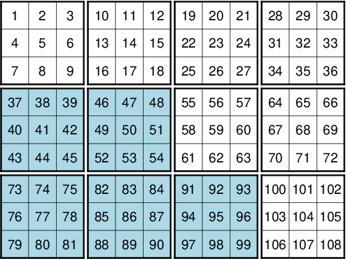
Grid split into 3 by 3 chunks
Gridded datasets in the earth sciences usually exhibit a strong spatial dependence (e.g. topography, potential fields, illustrated by blue and white cells in Figure Grid split into 3 by 3 chunks) and deflation can greatly reduce the file size and hence the file access time (deflating/inflating is faster than hard disk I/O). It is therefore convenient to deflate grids with spatial dependence (levels 1--3 give the best speed/size-tradeoff).
You may control the size of the chunks of data and compression with the configuration parameters IO_NC4_CHUNK_SIZE and IO_NC 4_DEFLATION_LEVEL as specified in gmt.conf and you can check the netCDF format with grdinfo.
Classic netCDF files were the de facto standard until netCDF 4.0 was released in 2008. Most programs supporting netCDF by now are using the netCDF-4 library and are thus capable of reading netCDF files generated with GMT 5, this includes official GMT releases since revision 4.5.8. In rare occasions, when you have to load netCDF files with old software, you may be forced to export your grids in the old classic format. This can be achieved by setting IO_NC4_CHUNK_SIZE to classic.
Further reading:
18.2.3. Gridline and Pixel node registration
Scanline format means that the data are stored in rows (y = constant) going from the “top” (\(y = y_{max}\) (north)) to the “bottom” (\(y = y_{min}\) (south)). Data within each row are ordered from “left” (\(x = x_{min}\) (west)) to “right” (\(x = x_{max}\) (east)). The registration signals how the nodes are laid out. The grid is always defined as the intersections of all x ( \(x = x_{min}, x_{min} + x_{inc}, x_{min} + 2 \cdot x_{inc}, \ldots, x_{max}\) ) and y ( \(y = y_{min}, y_{min} + y_{inc}, y_{min} + 2 \cdot y_{inc}, \ldots, y_{max}\) ) lines. The two scenarios differ as to which area each data point represents. The default node registration in GMT is gridline node registration. Most programs can handle both types, and for some programs like grdimage a pixel registered file makes more sense. Utility programs like grdsample and grdproject will allow you to convert from one format to the other; grdedit can make changes to the grid header and convert a pixel- to a gridline-registered grid, or vice versa. The grid registration is determined by the common GMT -r option (see Section Grid registration: The -r option).
18.2.4. Boundary Conditions for operations on grids
GMT has the option to specify boundary conditions in some programs that operate on grids (e.g., grdsample, grdgradient, grdtrack, nearneighbor, and grdview, to name a few. The desired condition can be set with the common GMT option -n; see Section Grid interpolation parameters: The -n option. The boundary conditions come into play when interpolating or computing derivatives near the limits of the region covered by the grid. The default boundary conditions used are those which are “natural” for the boundary of a minimum curvature interpolating surface. If the user knows that the data are periodic in x (and/or y), or that the data cover a sphere with x,y representing longitude,latitude, then there are better choices for the boundary conditions. Periodic conditions on x (and/or y) are chosen by specifying x (and/or y) as the boundary condition flags; global spherical cases are specified using the g (geographical) flag. Behavior of these conditions is as follows:
- Periodic
- conditions on x indicate that the data are periodic in the distance (\(x_{max} - x_{min}\)) and thus repeat values after every \(N = (x_{max} - x_{min})/x_{inc}\). Note that this implies that in a grid-registered file the values in the first and last columns are equal, since these are located at \(x = x_{min}\) and \(x = x_{max}\), and there are N + 1 columns in the file. This is not the case in a pixel-registered file, where there are only N and the first and last columns are located at \(x_{min} + x_{inc}/2\) and \(x_{max} - x_{inc}/2\). If y is periodic all the same holds for y.
- Geographical
conditions indicate the following:
- If \((x_{max} - x_{min}) \geq 360\) and also 180 modulo \(x_{inc} = 0\) then a periodic condition is used on x with a period of 360; else a default condition is used on the x boundaries.
- If condition 1 is true and also \(y_{max} = 90\) then a “north pole condition” is used at \(y_{max}\), else a default condition is used there.
- If condition 1 is true and also \(y_{min} = -90\) then a “south pole condition” is used at \(y_{min}\), else a default condition is used there.
“Pole conditions” use a 180º phase-shift of the data, requiring 180 modulo \(x_{inc} = 0\).
- Default
boundary conditions are
\[\nabla^2 f = \frac{\partial}{\partial n} \nabla^2 f = 0\]on the boundary, where \(f(x, y)\) is represented by the values in the grid file, and \(\partial/\partial n\) is the derivative in the direction normal to a boundary, and
\[\nabla^2 = \left(\frac{\partial^2}{\partial x^2} + \frac{\partial^2}{\partial y^2}\right)\]is the two-dimensional Laplacian operator.
18.2.5. Native binary grid files
The old-style native grid file format that was common in earlier version of GMT is still supported, although the use of netCDF files is strongly recommended. The file starts with a header of 892 bytes containing a number of attributes defining the content. The grdedit utility program will allow you to edit parts of the header of an existing grid file. The attributes listed in Table grdheader are contained within the header record in the order given (except the z-array which is not part of the header structure, but makes up the rest of the file). As this header was designed long before 64-bit architectures became available, the jump from the first three integers to the subsequent doubles in the structure does not occur on a 16-byte alignment. While GMT handles the reading of these structures correctly, enterprising programmers must take care to read this header correctly (see our code for details).
| Parameter | Description |
|---|---|
| int n_columns | Number of nodes in the x-dimension |
| int n_rows | Number of nodes in the y-dimension |
| int registration | 0 for grid line registration, 1 for pixel registration |
| double x_min | Minimum x-value of region |
| double x_max | Maximum x-value of region |
| double y_min | Minimum y-value of region |
| double y_max | Maximum y-value of region |
| double z_min | Minimum z-value in data set |
| double z_max | Maximum z-value in data set |
| double x_inc | Node spacing in x-dimension |
| double y_inc | Node spacing in y-dimension |
| double z_scale_factor | Factor to multiply z-values after read |
| double z_add_offset | Offset to add to scaled z-values |
| char x_units[80] | Units of the x-dimension |
| char y_units[80] | Units of the y-dimension |
| char z_units[80] | Units of the z-dimension |
| char title[80] | Descriptive title of the data set |
| char command[320] | Command line that produced the grid file |
| char remark[160] | Any additional comments |
| float z[n_columns*n_rows] | 1-D array with z-values in scanline format |
18.3. Sun raster files
The Sun raster file format consists of a header followed by a series of unsigned 1-byte integers that represents the bit-pattern. Bits are scanline oriented, and each row must contain an even number of bytes. The predefined 1-bit patterns in GMT have dimensions of 64 by 64, but other sizes will be accepted when using the -Gp|P option. The Sun header structure is outline in Table sunheader.
| Parameter | Description |
|---|---|
| int ras_magic | Magic number |
| int ras_width | Width (pixels) of image |
| int ras_height | Height (pixels) of image |
| int ras_depth | Depth (1, 8, 24, 32 bits) of pixel |
| int ras_length | Length (bytes) of image |
| int ras_type | Type of file; see RT_ below |
| int ras_maptype | Type of colormap; see RMT_ below |
| int ras_maplength | Length (bytes) of following map |
After the header, the color map (if ras_maptype is not RMT_NONE) follows for ras_maplength bytes, followed by an image of ras_length bytes. Some related definitions are given in Table sundef.
| Macro name | Description |
|---|---|
| RAS_MAGIC | 0x59a66a95 |
| RT_STANDARD | 1 (Raw pixrect image in 68000 byte order) |
| RT_BYTE_ENCODED | 2 (Run-length compression of bytes) |
| RT_FORMAT_RGB | 3 ([X]RGB instead of [X]BGR) |
| RMT_NONE | 0 (ras_maplength is expected to be 0) |
| RMT_EQUAL_RGB | 1 (red[ras_maplength/3],green[],blue[]) |
Numerous public-domain programs exist, such as xv and convert (in the GraphicsMagick or ImageMagick package), that will translate between various raster file formats such as tiff, gif, jpeg, and Sun raster. Raster patterns may be created with GMT plotting tools by generating PostScript plots that can be rasterized by ghostscript and translated into the right raster format.
19. Including GMT Graphics into your Documents
Now that you made some nice graphics with GMT, it is time to add them to a document, an article, a report, your dissertation, a poster, a web page, or a presentation. Of course, you could try the old-fashioned scissors and glue stick. More likely, you want to incorporate your graphics electronically into the document. Depending on the application, the GMT PostScript file will need to be converted to Encapsulated PostScript (EPS), Portable Document Format (PDF), or some raster format (e.g., JPEG, PNG, or TIFF) in order to incorporate them into the document.
- When creating a document intended for printing (article, dissertation, or poster) it is best to preserve the scalable vector characteristics of the PostScript file. Many applications can directly incorporate PostScript in the form of EPS files. Modern programs will often allow the inclusion of PDF files. Either way, the sharpness of lines and fonts will be preserved and can be scaled up or down as required.
- When the aim is to display the graphics on a computer screen or present it using a projector, it is wise to convert the PostScript into a raster format. Although applications like PowerPoint can do this for you, you can best take the conversion into your own hands for the best results.
A large number of questions to the GMT-Help mailing list are related to these rendering issues, showing that something as seemingly straightforward as incorporating a PostScript file into a document is a far from trivial exercise. This Chapter will show how to include GMT graphics into documents and how to achieve the best quality results.
19.1. Making GMT Encapsulated PostScript Files
GMT produces freeform PostScript files. Note that a freeform
PostScript file may contain special operators (such as
Setpagedevice) that is specific to printers (e.g., selection of
paper tray). Some previewers may not
understand these valid instructions and may fail to image the file.
Also, embedding freeform PostScript with such instructions in it into
a larger document can cause printing to fail. While you could choose
another viewer (we recommend ghostview) to view single plots
prepared by GMT, it is generally wiser to convert PostScript to EPS
output when you are creating a plot intended for inclusion into a larger
document. Some programs (and some publishers as well) do not allow the
use of instructions like Setpagedevice as part of embedded graphics.
An EPS file that is to be placed into another document needs to have correct bounding box parameters. These are found in the PostScript Document Comment %%BoundingBox. Applications that generate EPS files should set these parameters correctly. Because GMTmakes the PostScript files on the fly, often with several overlays, it is not possible to do so accurately. Therefore, if you need and EPS version with a “tight” BoundingBox you need to post-process your PostScript file. There are several ways in which this can be accomplished.
Programs such as Adobe Illustrator, Aldus Freehand, and Corel Draw will allow you to edit the BoundingBox graphically.
A command-line alternative is to use freely-available program epstool from the makers of Aladdin ghostscript. Running
epstool -c -b myplot.ps
should give a tight BoundingBox; epstool assumes the plot is page size and not a huge poster.
Another option is to use ps2epsi which also comes with the ghostscript package. Running
ps2epsi myplot.ps myplot.eps
should also do the trick. The downside is that this program adds an “image” of the plot in the preamble of the EPS file, thus increasing the file size significantly. This image is a rough rendering of your PostScript graphics that some programs will show on screen while you are editing your document. This image is basically a placeholder for the PostScript graphics that will actually be printed.
However, the preferred option is to use the GMT utility psconvert. Its -A option will figure out the tightest BoundingBox, again using ghostscript in the background. For example, running
gmt psconvert -A -Te myplot.ps
will convert the PostScript file
myplot.psinto an encapsulated PostScript filemyplot.epswhich is exactly cropped to the tightest possible BoundingBox.
If you do not want to modify your illustration but just include it in a text document: many word processors (such as Microsoft Word or Apple Pages) will let you include a PostScript file that you may place but not edit. Newer versions of those programs also allow you to include PDF versions of your graphics. Except for Pages, you will not be able to view the EPS figure on-screen, but it will print correctly.
19.2. Converting GMT PostScript to PDF or raster images
Since Adobe’s PDF (Portable Document Format) seems to have become the de facto standard for vector graphics, you are often well off converting GMT produced PostScript files to PDF. Being both vector formats (i.e., they basically describe all objects, text and graphics as lines and curves), such conversion sounds awfully straightforward and not worth a full section in this document. But experience has shown differently, since most converters cut corners by using the same tool (Aladdin’s ghostscript) with basic default options that are not devised to produce the best quality PDF files.
For some applications it is practical or even essential that you convert your PostScript file into a raster format, such as GIF (Graphics Interchange Format), TIFF (Tagged Image File Format), PNG (Portable Network Graphics), or JPEG (Joint Photographic Experts Group). A web page is better served with a raster image that will immediately show on a web browser, than with a PostScript file that needs to be downloaded to view, despite the better printing quality of the PostScript image. A less obvious reason to convert your image to a raster format is to by-pass PowerPoint’s rendering engine in case you want to embed the image into a presentation.
The are a number of programs that will convert PostScript files to PDF or raster formats, like Aladdin’s pstopdf, pbmplus’ pstoimg, or GraphicsMagick’s and ImageMagick’s convert, most of which run ghostscript behind the scenes. The same is true for viewers like ghostview and Apple’s Preview. So a lot of the times when people report that their PostScript plot does not look right but prints fine, it is the way ghostscript is used with its most basic settings that is to blame.
19.2.1. When converting or viewing PostScript goes awry
Here are some notorious pitfalls with ghostscript (and other rendering programs for that matter).
- Rendering.
- When you are converting to a raster format, make sure you use a high enough resolution so that the pixels do not show when it is enlarged onto a screen or using a projector. The right choice of resolution depends on the application, but do not feel limited to the default 72 dpi (dots-per-inch) that is offered by most converters.
- Image compression.
- There are lossy and non-lossy compressions. A compression algorithm is called “lossy” when information is lost in the conversion: there is no way back to get the full original. The effect can be seen when there are sharp color transitions in your image: the edges will get blurry in order to allow a more efficient compression. JPEG uses a lossy compression, PNG is non-lossy, and TIFF generally does not use compression at all. We therefore recommend you convert to PNG if you need to rasterize your plot, and leave JPEG to photographs.
- Embedded image compression.
- When your GMT plot includes objects produced by grdimage, psimage or pslegend, they are seen as “images”. The default options of ghostscript will use a lossy compression (similar to JPEG) on those images when converting them to PDF objects. This can be avoided, however, by inhibiting the compression altogether, or using the non-lossy flate compression, similar to the one used in the old compress program. This compression is fully reversible, so that your image does not suffer any loss.
- Auto-rotation.
- The ghostscript engine has the annoying habit to automatically rotate an image produced with portrait orientation (using the -P option) so that the height is always larger than the width. So if you have an image that was printed in portrait mode but happens to have a width larger than height (for example a global map), it would suddenly get rotated. Again, this function needs to be switched off. Apple’s Preview uses the ghostscript engine and suffers from the same annoying habit. Oddly enough, ghostscript does not force landscape plots to be “horizontal”.
- Anti-aliasing.
This is not something to worry about when converting to PDF, but certainly when producing raster images (discussed below). Anti-aliasing in this context means that the rendering tries to avoid aliasing, for example, sampling only the blacks in a black-and-white hachure. It does so by first oversampling the image and then using “gray-shades” when a target pixel is only partially white or black.
Clearly, this can lead to some unwanted results. First, all edges and lines get blurry and second, the assumption of a white background causes the gray shades to stand out when transferring the image to background with a different color (like the popular sleep-inducing blue in PowerPoint presentations). A more surprising effect of anti-aliasing is that the seams between tiles that make up the land mask when using pscoast will become visible. The anti-aliasing somehow decides to blur the edges of all polygons, even when they are seamlessly connected to other polygons.
It is therefore wise to overrule the default anti-aliasing option and over-sample the image yourself by choosing a higher resolution.
- Including fonts.
- When you are producing print-ready copy to publishers, they will often (and justifiably) ask that you include all fonts in your PDF document. Again, ghostscript (and all converters relying on that engine) will not do so by default.
19.2.2. Using psconvert
The remedy to all the problems mentioned in the previous section is readily available to you in the form of the GMT utility psconvert. It is designed to provide the best quality PDF and raster files using ghostscript as a rendering engine. The program psconvert avoids anti-aliasing and lossy compression techniques that are default to ghostscript and includes the fonts into the resulting PDF file to ensure portability. By default the fonts are rendered at 720 dots-per-inch in a PDF file and images are sampled to 300 dpi, but that can be changed with the -E option. Simply run
gmt psconvert -A -P -Tf *.ps
to convert all PostScript files to PDF while cropping it to the smallest possible BoundingBox. Or use the -Tg option to convert your files to PNG.
The -P option of psconvert may also come in handy. When you have not supplied the -P option in your first GMT plot command, your plot will be in Landscape mode. That means that the plot will be rotated 90º (anti-clockwise) to fit on a Portrait mode page when coming out of the printer. The -P option of psconvert will undo that rotation, so that you do not have to do so within your document. This will only affect Landscape plots; Portrait plots will not be rotated. We should note that the -A option in psconvert has many modifiers that can be used to control background color, framing, padding, and overall scaling of the result.
19.3. Examples
19.3.1. GMT graphics in LaTeX
To add the graphics into a LaTeX document we use the
\includegraphics command supplied by the package. In the preamble of
your LaTeX document you will need to include the line
\usepackage{graphicx}
The inclusion of the graphics will probably be inside a floating figure environment; something like this
\begin{figure}
   \includegraphics{myplot}
   \caption{This is my first plot in \LaTeX.}
   \label{fig:myplot}
\end{figure}
Note that the \includegraphics command does not require you to add
the suffix .pdf to the file name. If you run pdflatex, it will
look automatically for myplot.pdf. If you run latex, it will use myplot.eps instead.
You can scale your plot using the options width=, height=, or
scale=. In addition, if your original graphics was produced in
Landscape mode (i.e., you did not use GMT’s -P option: not
while plotting, nor in psconvert),
you will need to rotate the plot as well. For example,
\includegraphics[angle=-90,width=0.8\textwidth]{myplot}
will rotate the image 90º clockwise and scale it such that its width (after rotation) will be 80% of the width of the text column.
19.3.2. GMT graphics in PowerPoint
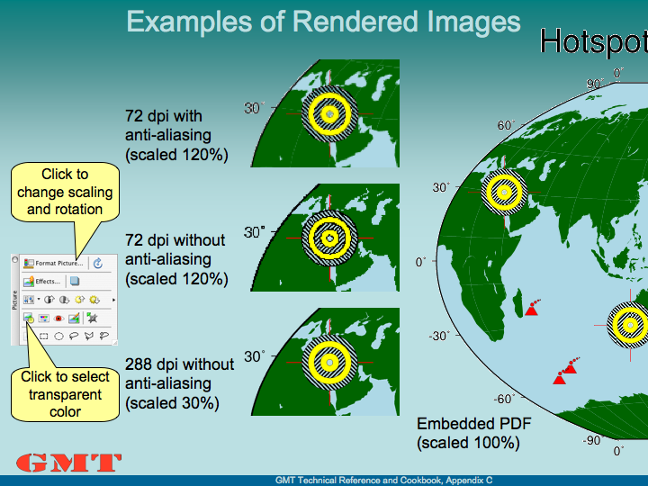
Examples of rendered images in a PowerPoint presentation
PowerPoint’s Format Picture dialogue to set scale and rotation.
In Figure Rendered images we have attempted to include Example (20) Custom plot symbols into a PowerPoint presentation. First the PostScript file was converted to PDF (using psconvert), then loaded into PowerPoint and the white background color was made transparent using the formatting toolbar (shown on the left side of Figure Rendered images). Clearly, when we let PowerPoint do the rendering, we do not get the best result:
- The anti-aliasing causes the tiles that make up the land to stand out. This is because the anti-aliasing algorithm blurs all edges, even when the tiles join seamlessly.
- The background color was assumed to be white, hence the text is “smoothed” using gray shades. Instead, shades of blue which would be appropriate for the background we are using.
On the central column of Figure Rendered images we have included PNG versions of a portion of the same example. This shows the workings of anti-aliasing and different resolutions. All samples were obtained with convert. The one on the top uses all default settings, resulting in an anti-aliased image at 72 dpi resolution (very much like the PDF included directly into PowerPoint).
Just switching anti-aliasing off (middle) is clearly not an option either. It is true that we got rid of the gray blurring and the seams between the tiles, but without anti-aliasing the image becomes very blocky. The solution is to render the image at a higher resolution (e.g., 300 dpi) without anti-aliasing and then shrink the image to the appropriate size (bottom of the central column in Figure Rendered images). The scaling, rotation as well as the selection of the transparent color can be accomplished through the “Formatting” tool bar and the “Format Picture” dialogue box of PowerPoint (Figure PowerPoint dialogue box), which can be found by double clicking the included image (or selecting and right-clicking or control-clicking on a one-button mouse).
19.4. Concluding remarks
These examples do not constitute endorsements of the products mentioned above; they only represent our limited experience with adding PostScript to various types of documents. For other solutions and further help, please post messages to the GMT user forum.
20. Predefined Bit and Hachure Patterns in GMT
GMT provides 90 different bit and hachure patterns that can be selected with the -Gp or -GP option in most plotting programs. The left side of each image was created using -Gp, the right side shows the inverted version using -GP. These patterns are reproduced below at 300 dpi using the default black and white shades.
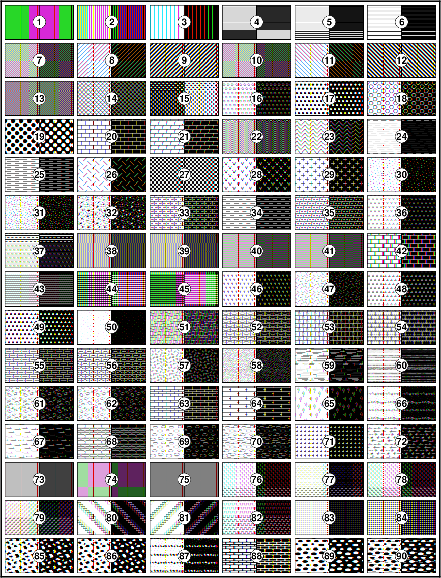
21. Chart of Octal Codes for Characters
The characters and their octal codes in the Standard and ISOLatin1 encoded fonts are shown in Figure Octal codes for Standard and ISO. Light red areas signify codes reserved for control characters. In order to use all the extended characters (shown in the light green boxes) you need to set PS_CHAR_ENCODING to Standard+ or ISOLatin1+ in your gmt.conf file [34].
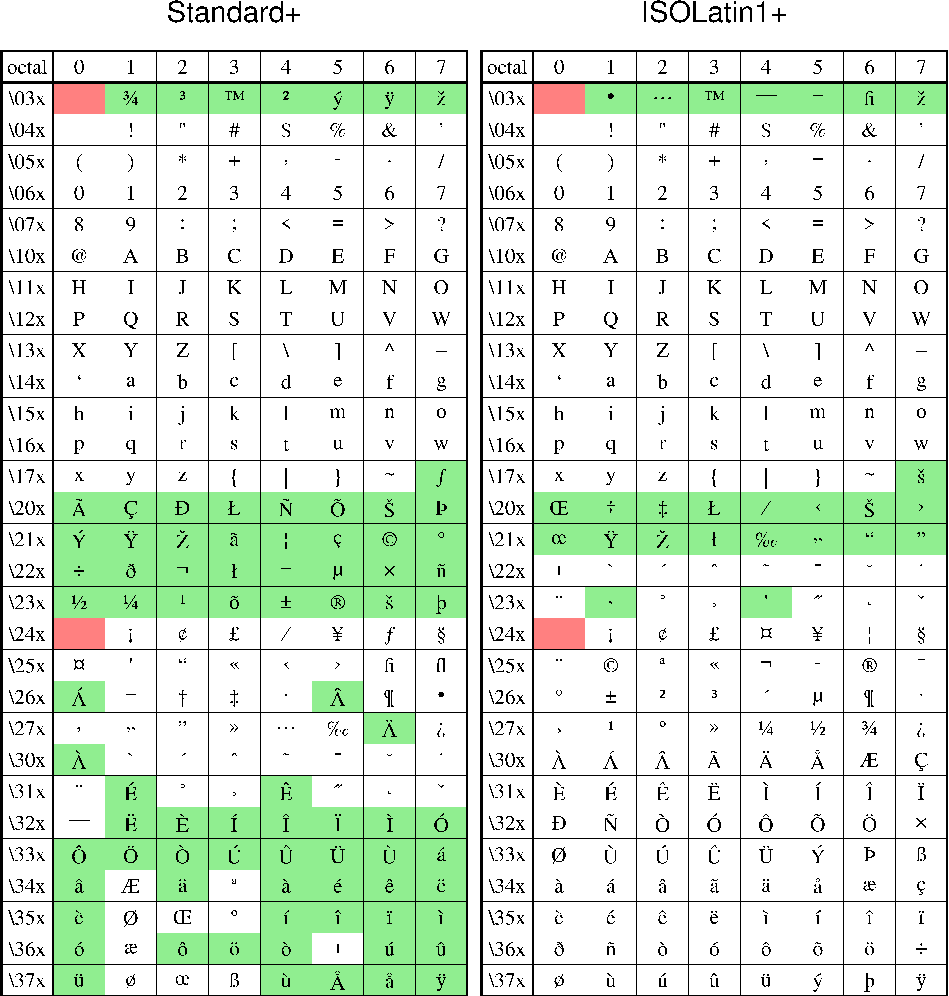
Octal codes and corresponding symbols for StandardEncoding (left) and ISOLatin1Encoding (right) fonts.
The chart for the Symbol character set (GMT font number 12) and Pifont ZapfDingbats character set (font number 34) are presented in Figure Octal codes for Symbol and ZapfDingbats below. The octal code is obtained by appending the column value to the \?? value, e.g., \(\partial\) is \266 in the Symbol font. The euro currency symbol is \240 in the Symbol font and will print if your printer supports it (older printer’s firmware will not know about the euro).
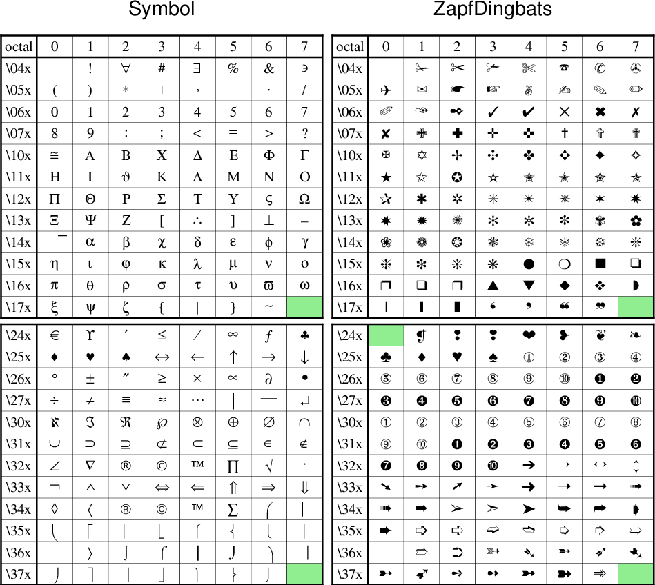
Octal codes and corresponding symbols for Symbol (left) and ZapfDingbats (right) fonts.
22. PostScript Fonts Used by GMT
GMT uses the standard 35 fonts that come with most PostScript laserwriters. If your printer does not support some of these fonts, it will automatically substitute the default font (which is usually Courier). The following is a list of the GMT fonts:
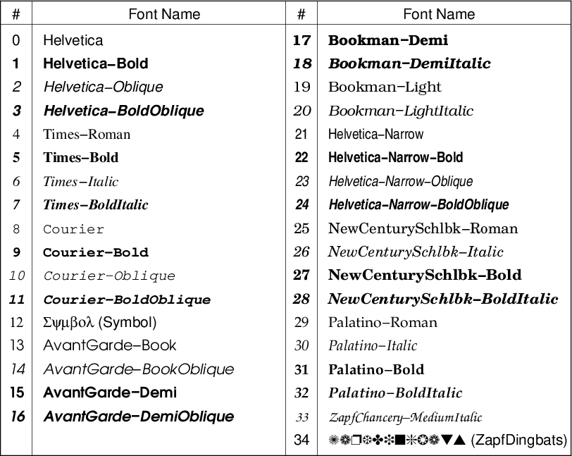
The standard 35 PostScript fonts recognized by GMT.
For the special fonts Symbol (12) and ZapfDingbats (34), see the octal charts in Chapter Chart of Octal Codes for Characters. When specifying fonts in GMT, you can either give the entire font name or just the font number listed in this table. To change the fonts used in plotting basemap frames, see the man page for gmt.conf. For direct plotting of text-strings, see the man page for pstext.
22.1. Using non-default fonts with GMT
To add additional fonts that you may have purchased or that are
available freely in the internet or at your institution, see the
instructions in the PSL_custom_fonts.txt under the share/postscriptlight directory and continue reading. GMT does
not read or process any font files and thus does not know anything about
installed fonts and their metrics. In order to use extra fonts in
GMT you need to specify the PostScript name of the relevant fonts in
the file PSL_custom_fonts.txt. You can either edit the existing file distributed with
GMT to make the changes global or you can create a new file in the
current working directory, e.g.,
LinBiolinumO      0.700    0
LinLibertineOB    0.700    0
The format is a space delimited list of the PostScript font name, the font height-point size-ratio, and a boolean variable that tells GMT to re-encode the font (if set to zero). The latter has to be set to zero as additional fonts will most likely not come in standard PostScript encoding. GMT determines how tall typical annotations might be from the font size ratio so that the vertical position of labels and titles can be adjusted to a more uniform typesetting. Now, you can set the GMT font parameters to your non-standard fonts:
gmt set FONT              LinBiolinumO \
        FONT_TITLE        28p,LinLibertineOB \
        PS_CHAR_ENCODING  ISO-8859-1 \
        MAP_DEGREE_SYMBOL degree
After setting the encoding and the degree symbol, the configuration part for GMT is finished and you can proceed to create GMT-maps as usual. An example script is discussed in Example (31) Using non-default fonts in PostScript.
22.1.1. Embedding fonts in PostScript and PDF
If you have Type 1 fonts in PFA (Printer Font ASCII) format you can embed them directly by copying them at the very top of your PostScript file, before even the %!PS header comment. PFB (Printer Font Binary), TrueType or OpenType fonts cannot be embedded in PostScript directly and therefore have to be converted to PFA first.
However, you most likely will have to tell Ghostscript where to
find your custom fonts in order to convert your GMT PostScript plot
to PDF or an image with psconvert.
When you have used the correct PostScript names of the fonts in PSL_custom_fonts.txt you
only need to point the GS_FONTPATH environment variable to the
directory where the font files can be found and invoke
psconvert in the usual way. Likewise
you can specify Ghostscript’s -sFONTPATH option on the
command line with C -sFONTPATH=/path/to/fontdir. Ghostscript,
which is invoked by psconvert, does
not depend on file names. It will automatically find the relevant font
files by their PostScript names and embed and subset them in
PDF-files. This is quite convenient as the document can be displayed and
printed even on other computers when the font is not available locally.
There is no need to convert your fonts as Ghostscript can handle
all Type 1, TrueType and OpenType fonts. Note also, that you do not need
to edit Ghostscript’s Fontmap.
If you do not want or cannot embed the fonts you can convert them to outlines (shapes with fills) with Ghostscript in the following way:
gs -q -dNOCACHE -dSAFER -dNOPAUSE -dBATCH -dNOPLATFONTS \
   -sDEVICE=ps2write -sFONTPATH="/path/to/fontdir" \
   -sOutputFile=mapWithOutlinedFonts.ps map.ps
Note, that this only works with the ps2write device. If you need outlined fonts in PDF, create the PDF from the converted PostScript file. Also, psconvert cannot correctly crop Ghostscript converted PostScript files anymore. Use Heiko Oberdiek’s instead or crop with psconvert -A -Te before (See Example (31) Using non-default fonts in PostScript).
22.1.2. Character encoding
Since PostScript itself does not support Unicode fonts, Ghostscript will re-encode the fonts on the fly. You have to make sure to set the correct PS_CHAR_ENCODING with gmtset and save your script file with the same character encoding. Alternatively, you can substitute all non ASCII characters with their corresponding octal codes, e.g., \265 instead of μ. Note, that PostScript fonts support only a small range of glyphs and you may have to switch the PS_CHAR_ENCODING within your script.
23. Color Space: The Final Frontier
In this Chapter, we are going to try to explain the relationship between the RGB, CMYK, and HSV color systems so as to (hopefully) make them more intuitive. GMT allows users to specify colors in CPTs in either of these three systems. Interpolation between colors is performed in either RGB or HSV, depending on the specification in the CPT. Below, we will explain why this all matters.
23.1. RGB color system
Remember your (parents’) first color television set? Likely it had three little bright colored squares on it: red, green, and blue. And that is exactly what each color on the tube is made of: varying levels of red, green and blue light. Switch all of them off, r=g=b=0, then you have black. All of them at maximum, r=g=b=255, creates white. Your computer screen works the same way.
A mix of levels of red, green, and blue creates basically any color imaginable. In GMT each color can be represented by the triplet r7g7b. For example, 127/255/0 (half red, full green, and no blue) creates a color called chartreuse. The color sliders in the graphics program GIMP are an excellent way to experiment with colors, since they show you in advance how moving one of the color sliders will change the color. As Figure (a) of Chartreuse in GIMP shows: increase the red and you will get a more yellow color, while lowering the blue level will turn it into brown.
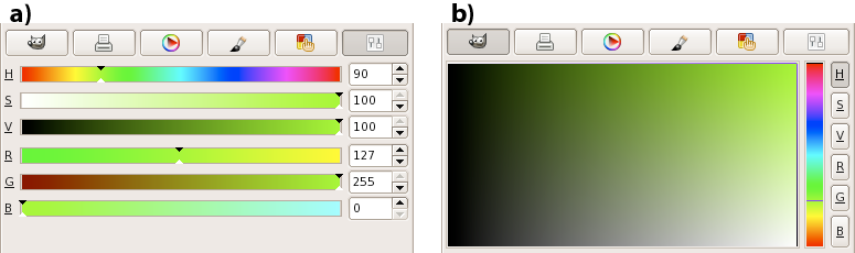
Chartreuse in GIMP. (a) Sliders indicate how the color is altered when changing the H, S, V, R, G, or B levels. (b) For a constant hue (here 90) value increases to the right and saturation increases up, so the pure color is on the top right.
Is chocolate your favorite color, but you do not know the RGB equivalent
values? Then look them up in Figure RGB chart or type
man gmtcolors for a full list. It’s 210/105/30. But GMT makes it easy
on you: you can specify pen, fill, and palette colors by any of the more
than 500 unique colors found in that file.
Are you very web-savvy and work best with hexadecimal color codes as
they are used in HTML? Even that is allowed in GMT. Just start with a
hash mark (#) and follow with the 2 hexadecimal characters for red,
green, and blue. For example, you can use #79ff00 for chartreuse,
#D2691E for chocolate.
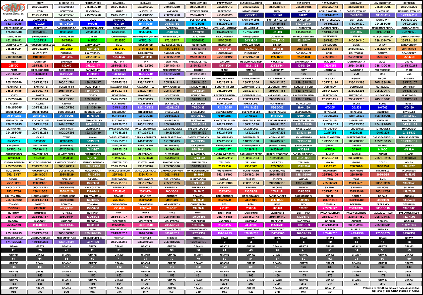
The 555 unique color names that can be used in GMT. Lower, upper, or mixed cases, as well as the british spelling of grey are allowed. A4, Letter, and Tabloid sized versions of this RGB chart can be found in the GMT documentation directory.
23.2. HSV color system
If you have played around with RGB color sliders, you will have noticed that it is not intuitive to make a chosen color lighter or darker, more saturated or more gray. It would involve changing three sliders. To make it easier to manipulate colors in terms of lightness and saturation, another coordinate system was invented: HSV (hue, saturation, value). Those terms can be made clear best by looking at the color sliders in Figure Chartreuse in GIMPa. Hue (running from 0 to 360) gives you the full spectrum of saturated colors. Saturation (from 0 to 1, or 100%) tells you how ‘full’ your color is: reduce it to zero and you only have gray scales. Value (from 0 to 1, or 100%) will bring you from black to a fully saturated color. Note that “value” is not the same as “intensity”, or “lightness”, used in other color geometries. “Brilliance” may be the best alternative word to describe “value”. Apple calls it as “brightness”, and hence refers to HSB for this color space.
Want more chartreuse or chocolate? You can specify them in GMT as 90-1-1 and 25-0.86-0.82, respectively.
23.3. The color cube
We are going to try to give you a geometric picture of color mixing in RGB and HSV by means of a tour of the RGB cube depicted in Figure The RGB color cube. The geometric picture is most helpful, we think, since HSV are not orthogonal coordinates and not found from RGB by a simple algebraic transformation. So here goes: Look at the cube face with black, red, magenta, and blue corners. This is the g = 0 face. Orient the cube so that you are looking at this face with black in the lower left corner. Now imagine a right-handed cartesian (rgb) coordinate system with origin at the black point; you are looking at the g = 0 plane with r increasing to your right, g increasing away from you, and b increasing up. Keep this sense of (rgb) as you look at the cube.
Now tip the cube such that the black corner faces down and the white corner up. When looking from the top, you can see the hue, contoured in gray solid lines, running around in 360º counter-clockwise. It starts with shades of red (0), then goes through green (120) and blue (240), back to red.
On the three faces that are now on the lower side (with the white print) one of (rgb) is equal to 0. These three faces meet at the black corner, where r = g = b = 0. On these three faces the colors are fully saturated: s = 1. The dashed white lines indicate different levels of v, ranging from 0 to 1 with contours every 0.1.
On the upper three faces (with the black print), one of (rgb) is equal to the maximum value. These three faces meet at the white corner, where r = g = b = 255. On these three faces value is at its maximum: v = 1 (or 100%). The dashed black lines indicate varying levels of saturation: s ranges from 0 to 1 with contours every 0.1.
Now turn the cube around on its vertical axis (running from the black to the white corner). Along the six edges that zigzag around the “equator”, both saturation and value are maximum, so s = v = 1. Twirling the cube around and tracing the zigzag, you will visit six of the eight corners of the cube, with changing hue (h): red (0), yellow (60), green (120), cyan (180), blue (240), and magenta (300). Three of these are the RGB colors; the other three are the CMY colors which are the complement of RGB and are used in many color hardcopy devices (see below). The only cube corners you did not visit on this path are the black and white corners. They lie on the vertical axis where hue is undefined and r = g = b. Any point on this axis is a shade of gray.
Let us call the points where s = v = 1 (points along the RYGCBM path described above) the “pure” colors. If we start at a pure color and we want to whiten it, we can keep h constant and v = 1 while decreasing s; this will move us along one of the cube faces toward the white point. If we start at a pure color and we want to blacken it, we can keep h constant and s = 1 while decreasing v; this will move us along one of the cube faces toward the black point. Any point in (rgb) space which can be thought of as a mixture of pure color + white, or pure color + black, is on a face of the cube.
The points in the interior of the cube are a little harder to describe. The definition for h above works at all points in (non-gray) (rgb) space, but so far we have only looked at (s, v) on the cube faces, not inside it. At interior points, none of (rgb) is equal to either 0 or 255. Choose such a point, not on the gray axis. Now draw a line through your point so that the line intersects the gray axis and also intersects the RYGCBM path of edges somewhere. It is always possible to construct this line, and all points on this line have the same hue. This construction shows that any point in RGB space can be thought of as a mixture of a pure color plus a shade of gray. If we move along this line away from the gray axis toward the pure color, we are “purifying” the color by “removing gray”; this move increases the color’s saturation. When we get to the point where we cannot remove any more gray, at least one of (rgb) will have become zero and the color is now fully saturated; s = 1. Conversely, any point on the gray axis is completely undersaturated, so that s = 0 there. Now we see that the black point is special, s is both 0 and 1 at the same time. In other words, at the black point saturation in undefined (and so is hue). The convention is to use h = s = v = 0 at this point.
It remains to define value. To do so, try this: Take your point in RGB space and construct a line through it so that this line goes through the black point; produce this line from black past your point until it hits a face on which v = 1. All points on this line have the same hue. Note that this line and the line we made in the previous paragraph are both contained in the plane whose hue is constant. These two lines meet at some arbitrary angle which varies depending on which point you chose. Thus HSV is not an orthogonal coordinate system. If the line you made in the previous paragraph happened to touch the gray axis at the black point, then these two lines are the same line, which is why the black point is special. Now, the line we made in this paragraph illustrates the following: If your chosen point is not already at the end of the line, where v = 1, then it is possible to move along the line in that direction so as to increase (rgb) while keeping the same hue. The effect this has on a color monitor is to make the color more “brilliant”, your hue will become “stronger”; if you are already on a plane where at least one of (rgb) = 255, then you cannot get a stronger version of the same hue. Thus, v measures brilliance or strength. Note that it is not quite true to say that v measures distance away from the black point, because v is not equal to \(\sqrt{r^2 + g^2 + b^2}/255\).
Another representation of the HSV space is the color cone illustrated in Figure The HSV color space.
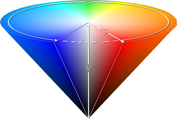
The HSV color space
23.4. Color interpolation
From studying the RGB cube, we hope you will have understood that there are different routes to follow between two colors, depending whether you are in the RGB or HSV system. Suppose you would make an interpolation between blue and red. In the RGB system you would follow a path diagonally across a face of the cube, from 0/0/255 (blue) via 127/0/127 (purple) to 255/0/0 (red). In the HSV system, you would trace two edges, from 240-1-1 (blue) via 300-1-1 (magenta) to 360-1-1 (red). That is even assuming software would be smart enough to go the shorter route. More likely, red will be recorded as 0-1-1, so hue will be interpolated the other way around, reducing hue from 240 to 0, via cyan, green, and yellow.
Depending on the design of your CPT, you may want to have it
either way. By default, GMT interpolates in RGB space, even when the
original CPT is in the HSV system. However, when you add the
line #COLOR_MODEL=+HSV (with the leading ‘+’ sign) in the header of
the CPT, GMT will not only read the color
representation as HSV values, but also interpolate colors in the HSV
system. That means that H, S, and V values are interpolated linearly
between two colors, instead of their respective R, G, and B values.
The top row in Figure Interpolating colors illustrates two examples: a blue-white-red scale (the palette in Chapter Of Colors and Color Legends) interpolated in RGB and the palette interpolated in HSV. The bottom row of the Figure demonstrates how things can go terribly wrong when you do the interpolation in the other system.
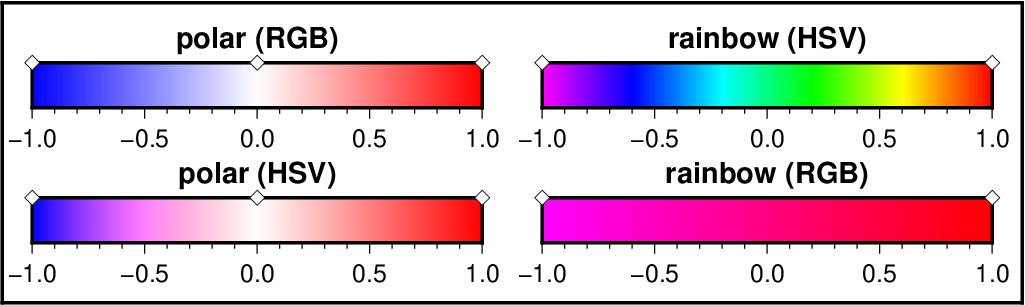
When interpolating colors, the color system matters. The polar palette on the left needs to be interpolated in RGB, otherwise hue will change between blue (240) and white (0). The rainbow palette should be interpolated in HSV, since only hue should change between magenta (300) and red (0). Diamonds indicate which colors are defined in the palettes; they are fixed, the rest is interpolated.
23.5. Artificial illumination
GMT uses the HSV system to achieve artificial illumination of colored images (e.g., -I option in grdimage) by changing the saturation s and value v coordinates of the color. When the intensity is zero (flat illumination), the data are colored according to the CPT. If the intensity is non-zero, the color is either lightened or darkened depending on the illumination. The color is first converted to HSV (if necessary) and then darkened by moving (sv) toward (COLOR_HSV_MIN_S, COLOR_HSV_MIN_V) if the intensity is negative, or lightened by sliding (sv) toward (COLOR_HSV_MAX_S, COLOR_HSV_MAX_V) if the illumination is positive. The extremes of the s and v are defined in the gmt.conf file and are usually chosen so the corresponding points are nearly black (s = 1, v = 0) and white (s = 0, v = 1). The reason this works is that the HSV system allows movements in color space which correspond more closely to what we mean by “tint” and “shade”; an instruction like “add white” is easy in HSV and not so obvious in RGB.
23.6. Thinking in RGB or HSV
The RGB system is understandable because it is cartesian, and we all learned cartesian coordinates in school. But it doesn’t help us create a tint or shade of a color; we cannot say, “We want orange, and a lighter shade of orange, or a less vivid orange”. With HSV we can do this, by saying, “Orange must be between red and yellow, so its hue is about h = 30; a less vivid orange has a lesser s, a darker orange has a lesser v”. On the other hand, the HSV system is a peculiar geometric construction, more like a cone (Figure The HSV color space). It is not an orthogonal coordinate system, and it is not found by a matrix transformation of RGB; these make it difficult in some cases too. Note that a move toward black or a move toward white will change both s and v, in the general case of an interior point in the cube. The HSV system also doesn’t behave well for very dark colors, where the gray point is near black and the two lines we constructed above are almost parallel. If you are trying to create nice colors for drawing chocolates, for example, you may be better off guessing in RGB coordinates.
23.7. CMYK color system
Finally, you can imagine that printers work in a different way: they mix different paints to make a color. The more paint, the darker the color, which is the reverse of adding more light. Also, mixing more colored paints does not give you true black, so that means that you really need four colors to do it right. Open up your color printer and you’ll probably find four cartridges: cyan, magenta, yellow (often these are combined into one), and black. They form the CMYK system of colors, each value running from 0 to 1 (or 100%). In GMT CMYK color coding can be achieved using c/m/y/k quadruplets.
Obviously, there is no unique way to go from the 3-dimensional RGB system to the 4-dimensional CMYK system. So, again, there is a lot of hand waving applied in the transformation. Strikingly, CMYK actually covers a smaller color space than RGB. We will not try to explain you the details behind it, just know that there is a transformation needed to go from the colors on your screen to the colors on your printer. It might explain why what you see is not necessarily what you get. If you are really concerned about how your color plots will show up in your PhD thesis, for example, it might be worth trying to save and print all your color plots using the CMYK system. Letting GMT do the conversion to CMYK may avoid some nasty surprises when it comes down to printing. To specify the color space of your PostScript file, set PS_COLOR_MODEL in the gmt.conf file to RGB, HSV, or CMYK.
24. Filtering of Data in GMT
The GMT programs filter1d (for tables of data indexed to one independent variable) and grdfilter (for data given as 2-dimensional grids) allow filtering of data by a moving-window process. (To filter a grid by Fourier transform use grdfft.) Both programs use an argument -F<type><width> to specify the type of process and the window’s width (in 1-D) or diameter (in 2-D). (In filter1d the width is a length of the time or space ordinate axis, while in grdfilter it is the diameter of a circular area whose distance unit is related to the grid mesh via the -D option). If the process is a median, mode, or extreme value estimator then the window output cannot be written as a convolution and the filtering operation is not a linear operator. If the process is a weighted average, as in the boxcar, cosine, and gaussian filter types, then linear operator theory applies to the filtering process. These three filters can be described as convolutions with an impulse response function, and their transfer functions can be used to describe how they alter components in the input as a function of wavelength.
Impulse responses are shown here for the boxcar, cosine, and gaussian filters. Only the relative amplitudes of the filter weights shown; the values in the center of the window have been fixed equal to 1 for ease of plotting. In this way the same graph can serve to illustrate both the 1-D and 2-D impulse responses; in the 2-D case this plot is a diametrical cross-section through the filter weights (Figure Impulse responses).
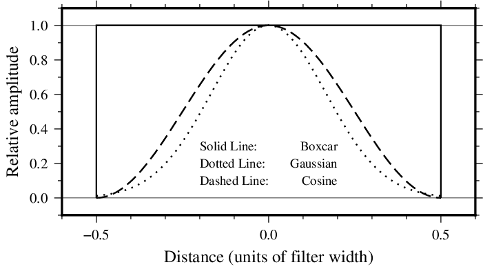
Impulse responses for GMT filters.
Although the impulse responses look the same in 1-D and 2-D, this is not true of the transfer functions; in 1-D the transfer function is the Fourier transform of the impulse response, while in 2-D it is the Hankel transform of the impulse response. These are shown in Figures Transfer functions for 1D and 2D, respectively. Note that in 1-D the boxcar transfer function has its first zero crossing at f = 1, while in 2-D it is around \(f \sim 1.2\). The 1-D cosine transfer function has its first zero crossing at f = 2; so a cosine filter needs to be twice as wide as a boxcar filter in order to zero the same lowest frequency. As a general rule, the cosine and gaussian filters are “better” in the sense that they do not have the “side lobes” (large-amplitude oscillations in the transfer function) that the boxcar filter has. However, they are correspondingly “worse” in the sense that they require more work (doubling the width to achieve the same cut-off wavelength).
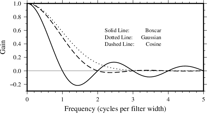
Transfer functions for 1-D GMT filters.
One of the nice things about the gaussian filter is that its transfer functions are the same in 1-D and 2-D. Another nice property is that it has no negative side lobes. There are many definitions of the gaussian filter in the literature (see page 7 of Bracewell [35]). We define \(\sigma\) equal to 1/6 of the filter width, and the impulse response proportional to \(\exp[-0.5(t/\sigma)^2)\). With this definition, the transfer function is \(\exp[-2(\pi\sigma f)^2]\) and the wavelength at which the transfer function equals 0.5 is about 5.34 \(\sigma\), or about 0.89 of the filter width.
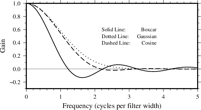
Transfer functions for 2-D (radial) GMT filters.
25. The GMT High-Resolution Coastline Data
Starting with version 3.0, GMT use a completely new coastline database and the pscoast utility was been completely rewritten to handle the new file format. Many users have asked us why it has taken so long for GMT to use a high-resolution coastline database; after all, such data have been available in the public domain for years. To answer such questions we will take you along the road that starts with these public domain data sets and ends up with the database used by GMT.
25.1. Selecting the right data
There are two well-known public-domain data sets that could be used for this purpose. Once is known as the World Data Bank II or CIA Data Bank (WDB) and contains coastlines, lakes, political boundaries, and rivers. The other, the World Vector Shoreline (WVS) only contains shorelines between saltwater and land (i.e., no lakes). It turns out that the WVS data is far superior to the WDB data as far as data quality goes, but as noted it lacks lakes, not to mention rivers and borders. We decided to use the WVS whenever possible and supplement it with WDB data. We got these data over the Internet; they are also available on CD-ROM from the National Geophysical Data Center in Boulder, Colorado [36].
25.2. Format required by GMT
In order to paint continents or oceans it is necessary that the coastline data be organized in polygons that may be filled. Simple line segments can be used to draw the coastline, but for painting polygons are required. Both the WVS and WDB data consists of unsorted line segments: there is no information included that tells you which segments belong to the same polygon (e.g., Australia should be one large polygon). In addition, polygons enclosing land must be differentiated from polygons enclosing lakes since they will need different paint. Finally, we want pscoast to be flexible enough that it can paint the land or the oceans or both. If just land (or oceans) is selected we do not want to paint those areas that are not land (or oceans) since previous plot programs may have drawn in those areas. Thus, we will need to combine polygons into new polygons that lend themselves to fill land (or oceans) only (Note that older versions of pscoast always painted lakes and wiped out whatever was plotted beneath).
25.3. The long and winding road
The WVS and WDB together represent more than 100 Mb of binary data and something like 20 million data points. Hence, it becomes obvious that any manipulation of these data must be automated. For instance, the reasonable requirement that no coastline should cross another coastline becomes a complicated processing step.
To begin, we first made sure that all data were “clean”, i.e., that there were no outliers and bad points. We had to write several programs to ensure data consistency and remove “spikes” and bad points from the raw data. Also, crossing segments were automatically “trimmed” provided only a few points had to be deleted. A few hundred more complicated cases had to be examined semi-manually.
Programs were written to examine all the loose segments and determine which segments should be joined to produce polygons. Because not all segments joined exactly (there were non-zero gaps between some segments) we had to find all possible combinations and choose the simplest combinations. The WVS segments joined to produce more than 200,000 polygons, the largest being the Africa-Eurasia polygon which has 1.4 million points. The WDB data resulted in a smaller data base (~25% of WVS).
We now needed to combine the WVS and WDB data bases. The main problem here is that we have duplicates of polygons: most of the features in WVS are also in WDB. However, because the resolution of the data differ it is nontrivial to figure out which polygons in WDB to include and which ones to ignore. We used two techniques to address this problem. First, we looked for crossovers between all possible pairs of polygons. Because of the crossover processing in step 1 above we know that there are no remaining crossovers within WVS and WDB; thus any crossovers would be between WVS and WDB polygons. Crossovers could mean two things: (1) A slightly misplaced WDB polygon crosses a more accurate WVS polygon, both representing the same geographic feature, or (2) a misplaced WDB polygon (e.g., a small coastal lake) crosses the accurate WVS shoreline. We distinguished between these cases by comparing the area and centroid of the two polygons. In almost all cases it was obvious when we had duplicates; a few cases had to be checked manually. Second, on many occasions the WDB duplicate polygon did not cross its WVS counterpart but was either entirely inside or outside the WVS polygon. In those cases we relied on the area-centroid tests.
While the largest polygons were easy to identify by visual inspection, the majority remain unidentified. Since it is important to know whether a polygon is a continent or a small pond inside an island inside a lake we wrote programs that would determine the hierarchical level of each polygon. Here, level = 1 represents ocean/land boundaries, 2 is land/lakes borders, 3 is lakes/islands-in-lakes, and 4 is islands-in-lakes/ponds-in-islands-in-lakes. Level 4 was the highest level encountered in the data. To automatically determine the hierarchical levels we wrote programs that would compare all possible pairs of polygons and find how many polygons a given polygon was inside. Because of the size and number of the polygons such programs would typically run for 3 days on a Sparc-2 workstation.
Once we know what type a polygon is we can enforce a common “orientation” for all polygons. We arranged them so that when you move along a polygon from beginning to end, your left hand is pointing toward “land”. At this step we also computed the area of all polygons since we would like the option to plot only features that are bigger than a minimum area to be specified by the user.
Obviously, if you need to make a map of Denmark then you do not want to read the entire 1.4 million points making up the Africa-Eurasia polygon. Furthermore, most plotting devices will not let you paint and fill a polygon of that size due to memory restrictions. Hence, we need to partition the polygons so that smaller subsets can be accessed rapidly. Likewise, if you want to plot a world map on a letter-size paper there is no need to plot 10 million data points as most of them will plot several times on the same pixel and the operation would take a very long time to complete. We chose to make 5 versions on the database, corresponding to different resolutions. The decimation was carried out using the Douglas-Peucker (DP) line-reduction algorithm [37]. We chose the cutoffs so that each subset was approximately 20% the size of the next higher resolution. The five resolutions are called full, high, intermediate, low, and crude; they are accessed in pscoast, gmtselect, and grdlandmask with the -D option [38]. For each of these 5 data sets (f, h, i, l, c) we specified an equidistant grid (1, 2, 5, 10, 20) and split all polygons into line-segments that each fit inside one of the many boxes defined by these grid lines. Thus, to paint the entire continent of Australia we instead paint many smaller polygons made up of these line segments and gridlines. Some book-keeping has to be done since we need to know which parent polygon these smaller pieces came from in order to prescribe the correct paint or ignore if the feature is smaller than the cutoff specified by the user. The resulting segment coordinates were then scaled to fit in short integer format to preserve precision and written in netCDF format for ultimate portability across hardware platforms [39].
While we are now back to a file of line-segments we are in a much better position to create smaller polygons for painting. Two problems must be overcome to correctly paint an area:
- We must be able to join line segments and grid cell borders into meaningful polygons; how we do this will depend on whether we want to paint the land or the oceans.
- We want to nest the polygons so that no paint falls on areas that are “wet” (or “dry”); e.g., if a grid cell completely on land contains a lake with a small island, we do not want to paint the lake and then draw the island, but paint the annulus or “donut” that is represented by the land and lake, and then plot the island.
GMT uses a polygon-assembly routine that carries out these tasks on the fly.
25.4. The Five Resolutions
We will demonstrate the power of the new database by starting with a regional hemisphere map centered near Papua New Guinea and zoom in on a specified point. The map regions will be specified in projected km from the projection center, e.g., we may want the map to go from km to km in the longitudinal and the latitudinal direction. Also, as we zoom in on the projection center we want to draw the outline of the next map region on the plot. To do that we use the -D option in psbasemap.
25.4.1. The crude resolution (-Dc)
We begin with an azimuthal equidistant map of the hemisphere centered on 130°21’E, 0°12’S, which is slightly west of New Guinea, near the Strait of Dampier. The edges of the map are all 9000 km true distance from the projection center. At this scale (and for global maps) the crude resolution data will usually be adequate to capture the main geographic features. To avoid cluttering the map with insignificant detail we only plot features (i.e., polygons) that exceed 500 km2 in area. Smaller features would only occupy a few pixels on the plot and make the map look “dirty”. We also add national borders to the plot. The crude database is heavily decimated and simplified by the DP-routine: The total file size of the coastlines, rivers, and borders database is only 283 kbytes. The plot is produced by the script:
gmt set MAP_GRID_CROSS_SIZE_PRIMARY 0 MAP_ANNOT_OBLIQUE 22 MAP_ANNOT_MIN_SPACING 0.3i
gmt pscoast -Rk-9000/9000/-9000/9000 -JE130.35/-0.2/3.5i -P -Dc -A500 \
            -Gburlywood -Sazure -Wthinnest -N1/thinnest,- -B20g20 -BWSne -K > GMT_App_K_1.ps
gmt psbasemap -R -J -O -Dk2000+c130.35/-0.2+pthicker >> GMT_App_K_1.ps
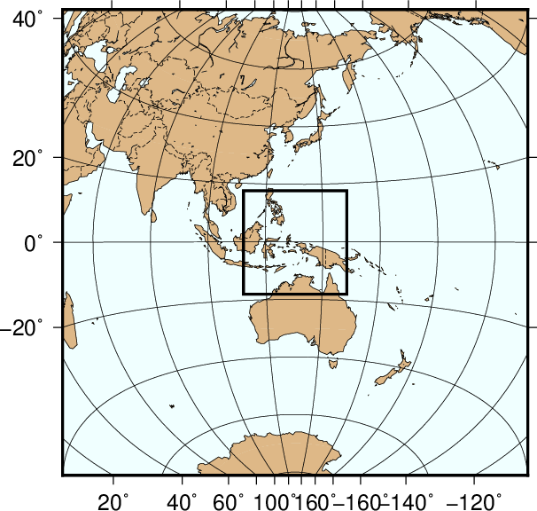
Map using the crude resolution coastline data.
Here, we use the MAP_ANNOT_OBLIQUE bit flags to achieve horizontal annotations and set MAP_ANNOT_MIN_SPACING to suppress some longitudinal annotations near the S pole that otherwise would overprint. The square box indicates the outline of the next map.
25.4.2. The low resolution (-Dl)
We have now reduced the map area by zooming in on the map center. Now, the edges of the map are all 2000 km true distance from the projection center. At this scale we choose the low resolution data that faithfully reproduce the dominant geographic features in the region. We cut back on minor features less than 100 km2 in area. We still add national borders to the plot. The low database is less decimated and simplified by the DP-routine: The total file size of the coastlines, rivers, and borders combined grows to 907 kbytes; it is the default resolution in GMT. The plot is generated by the script:
gmt pscoast -Rk-2000/2000/-2000/2000 -JE130.35/-0.2/3.5i -P -Dl -A100 -Gburlywood \
            -Sazure -Wthinnest -N1/thinnest,- -B10g5 -BWSne -K > GMT_App_K_2.ps
gmt psbasemap -R -J -O -Dk500+c130.35/-0.2+pthicker >> GMT_App_K_2.ps
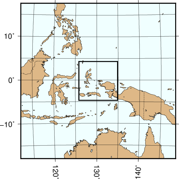
Map using the low resolution coastline data.
25.4.3. The intermediate resolution (-Di)
We continue to zoom in on the map center. In this map, the edges of the map are all 500 km true distance from the projection center. We abandon the low resolution data set as it would look too jagged at this scale and instead employ the intermediate resolution data that faithfully reproduce the dominant geographic features in the region. This time, we ignore features less than 20 km2 in area. Although the script still asks for national borders none exist within our region. The intermediate database is moderately decimated and simplified by the DP-routine: The combined file size of the coastlines, rivers, and borders now exceeds 3.35 Mbytes. The plot is generated by the script:
gmt pscoast -Rk-500/500/-500/500 -JE130.35/-0.2/3.5i -P -Di -A20 -Gburlywood \
            -Sazure -Wthinnest -N1/thinnest,- -B2g1 -BWSne -K > GMT_App_K_3.ps
echo 133 2 | gmt psxy -R -J -O -K -Sc1.4i -Gwhite >> GMT_App_K_3.ps
gmt psbasemap -R -J -O -K --FONT_TITLE=12p --MAP_TICK_LENGTH_PRIMARY=0.05i \
              -Tm133/2+w1i+t45/10/5+jCM --FONT_ANNOT_SECONDARY=8p >> GMT_App_K_3.ps
gmt psbasemap -R -J -O -Dk100+c130.35/-0.2+pthicker >> GMT_App_K_3.ps
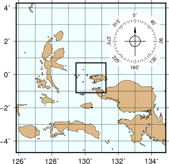
Map using the intermediate resolution coastline data. We have added a compass rose just because we have the power to do so.
25.4.4. The high resolution (-Dh)
The relentless zooming continues! Now, the edges of the map are all 100 km true distance from the projection center. We step up to the high resolution data set as it is needed to accurately portray the detailed geographic features within the region. Because of the small scale we only ignore features less than 1 km2 in area. The high resolution database has undergone minor decimation and simplification by the DP-routine: The combined file size of the coastlines, rivers, and borders now swells to 12.3 Mbytes. The map and the final outline box are generated by these commands:
gmt pscoast -Rk-100/100/-100/100 -JE130.35/-0.2/3.5i -P -Dh -A1 -Gburlywood \
            -Sazure -Wthinnest -N1/thinnest,- -B30mg10m -BWSne -K > GMT_App_K_4.ps
gmt psbasemap -R -J -O -Dk20+c130.35/-0.2+pthicker >> GMT_App_K_4.ps
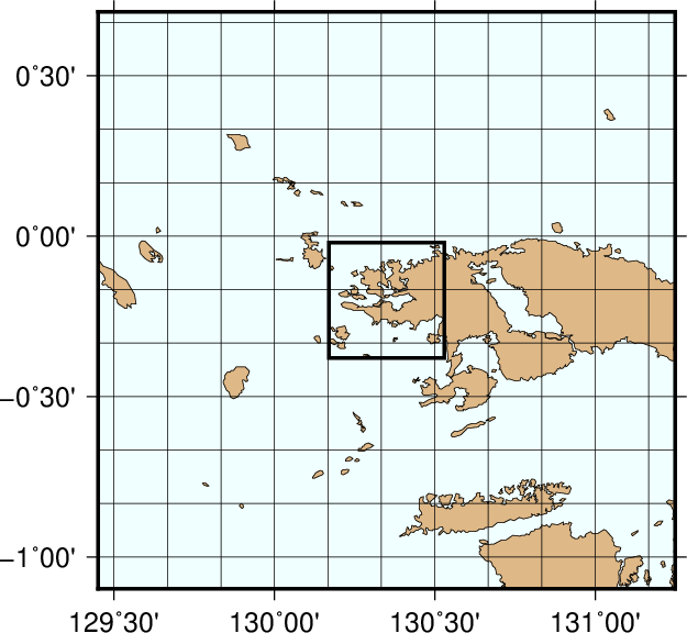
Map using the high resolution coastline data.
25.4.5. The full resolution (-Df)
We now arrive at our final plot, which shows a detailed view of the western side of the small island of Waigeo. The map area is approximately 40 by 40 km. We call upon the full resolution data set to portray the richness of geographic detail within this region; no features are ignored. The full resolution has undergone no decimation and it shows: The combined file size of the coastlines, rivers, and borders totals a (once considered hefty) 55.9 Mbytes. Our final map is reproduced by the single command:
gmt pscoast -Rk-20/20/-20/20 -JE130.35/-0.2/3.5i -P -Df -Gburlywood \
            -Sazure -Wthinnest -N1/thinnest,- -B10mg2m -BWSne > GMT_App_K_5.ps
Map using the full resolution coastline data.
We hope you will study these examples to enable you to make efficient and wise use of this vast data set.
26. GMT on non-UNIX Platforms
26.1. Introduction
While GMT was ported to non-UNIX systems such as Windows, it is also true that one of the strengths of GMT lies its symbiotic relationship with UNIX. We therefore recommend that GMT be installed in a POSIX-compliant UNIX environment such as traditional UNIX-systems, Linux, or Mac OS X. If abandoning your non-UNIX operating system is not an option, consider one of these solutions:
- WINDOWS:
Choose among these three possibilities:
- Install GMT under MinGW/MSYS (A collection of GNU utilities).
- Install GMT under Cygwin (A GNU port to Windows).
- Install GMT in Windows using Microsoft C/C++ or other compilers. Unlike the first two, this option will not provide you with any UNIX tools so you will be limited to what you can do with DOS batch files.
26.2. Cygwin and GMT
Because GMT works best in conjugation with UNIX tools we suggest you install GMT using the Cygwin product from Cygnus (now assimilated by Redhat, Inc.). This free version works on any Windows version and it comes with both the Bourne Again shell bash and the tcsh. You also have access to most standard GNU development tools such as compilers and text processing tools (awk, grep, sed, etc.). Note that executables prepared for Windows will also run under Cygwin.
Follow the instructions on the Cygwin page on how to install the package; note you must explicitly add all the development tool packages (e.g., gcc etc) as the basic installation does not include them by default. Once you are up and running under Cygwin, you may install GMT the same way you do under any other UNIX platform; our wiki has instructions for packages you need to install first.
Finally, from Cygwin’s User Guide: By default, no Cygwin program can allocate more than 384 MB of memory (program and data). You should not need to change this default in most circumstances. However, if you need to use more real or virtual memory in your machine you may add an entry in either the HKEY_LOCAL_MACHINE (to change the limit for all users) or HKEY_CURRENT_USER (for just the current user) section of the registry. Add the DWORD value heap_chunk_in_mb and set it to the desired memory limit in decimal Mb. It is preferred to do this in Cygwin using the regtool program included in the Cygwin package. (For more information about regtool or the other Cygwin utilities, see the Section called Cygwin Utilities in Chapter 3 of the Cygwin’s User Guide or use the help option of each utility.) You should always be careful when using regtool since damaging your system registry can result in an unusable system. This example sets the local machine memory limit to 1024 Mb:
regtool -i set /HKLM/Software/Cygnus\ Solutions/Cygwin/heap_chunk_in_mb 1024
regtool -v list /HKLM/Software/Cygnus\ Solutions/Cygwin
For more installation details see the general README file.
26.3. MINGW|MSYS and GMT
Though one can install GMT natively using CMake, the simplest way of installing under MINGW|MSYS is to just install the Windows binaries and use them from the msys bash shell. As simple as that. Furthermore, GMT programs launch faster here than on Cygwin so this is the recommended way of running GMT on Windows.
27. Of Colors and Color Legends
27.1. Built-in color palette tables (CPT)
Figures CPTs a and b show the 40 built-in color palettes, stored in so-called CPTs [40]. The programs makecpt and grd2cpt are used to access these master CPTs and translate/scale them to fit the user’s range of z-values. The top half of the color bars in the Figure shows the original color scale, which can be either discrete or continuous, though some (like globe) are a mix of the two. The bottom half the color bar are built by using makecpt -T-1/1/0.25, thus splitting the color scale into 8 discrete colors.
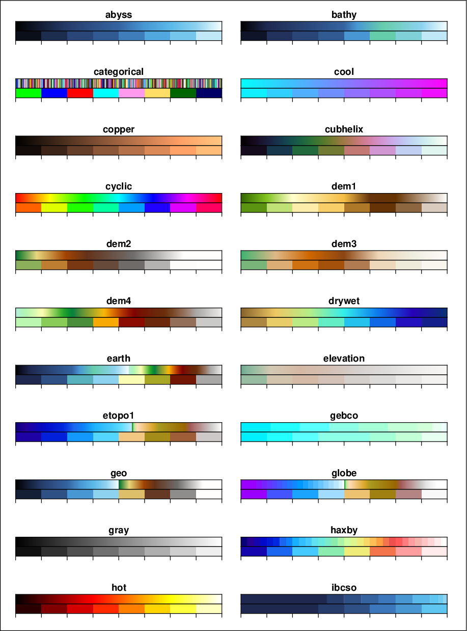
The first 22 of the standard 44 CPTs supported by GMT
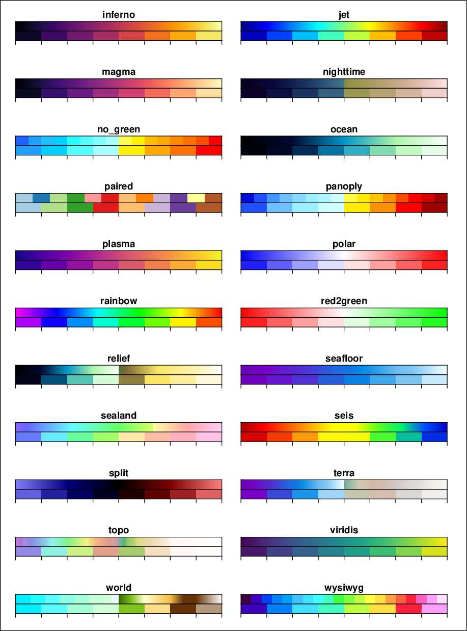
The second 22 of the standard 44 CPTs supported by GMT
27.2. Labeled and non-equidistant color legends
The use of color legends has already been introduced in Examples 2, 16, and 17. Things become a bit more complicated when you want to label the legend with names for certain intervals (like geological time periods in the example below). To accomplish that, one should add a semi-colon and the label name at the end of a line in the CPT and add the -L option to the psscale command that draws the color legend. This option also makes all intervals in the legend of equal length, even it the numerical values are not equally spaced.
Normally, the name labels are plotted at the lower end of the intervals. But by adding a gap amount (even when zero) to the -L option, they are centered. The example below also shows how to annotate ranges using -Li (in which case no name labels should appear in the CPT), and how to switch the color bar around (by using a negative length).
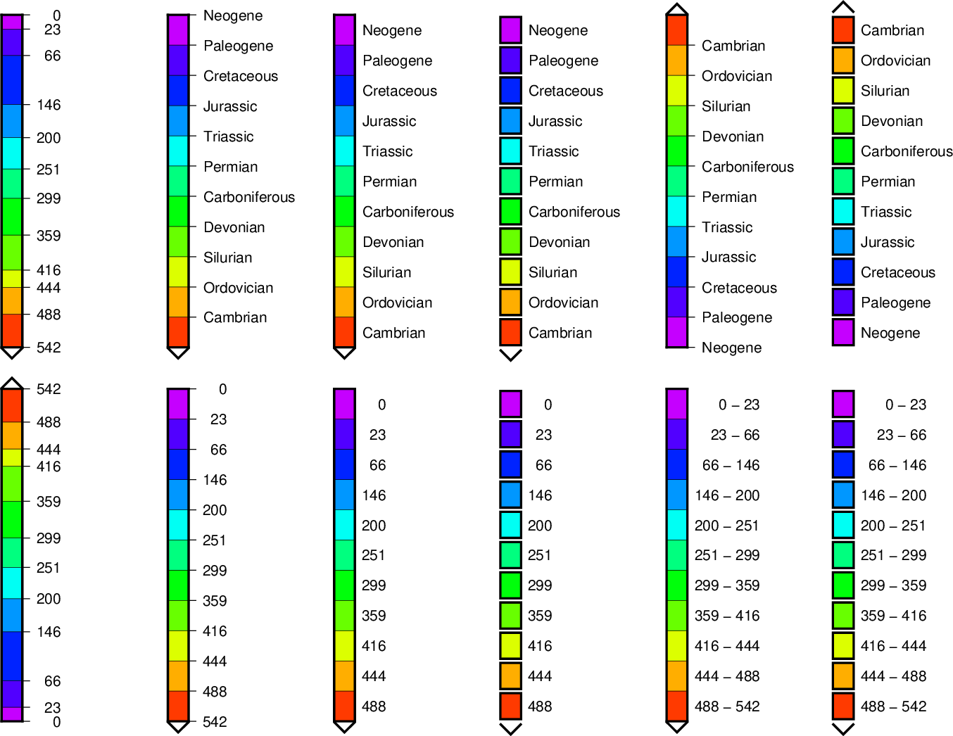
For additional color tables, visit cpt-city.
28. Custom Plot Symbols
28.1. Background
The GMT tools psxy and psxyz are capable of using custom
symbols as alternatives to the built-in, standard geometrical shapes
such as circles, triangles, and many others. One the command line, custom
symbols are selected via the -Sksymbolname[size] symbol
selection, where symbolname refers to a special symbol definition file
called symbolname.def that must be available via the standard GMT user paths. Several
custom symbols comes pre-configured with GMT (see
Figure Custom symbols)
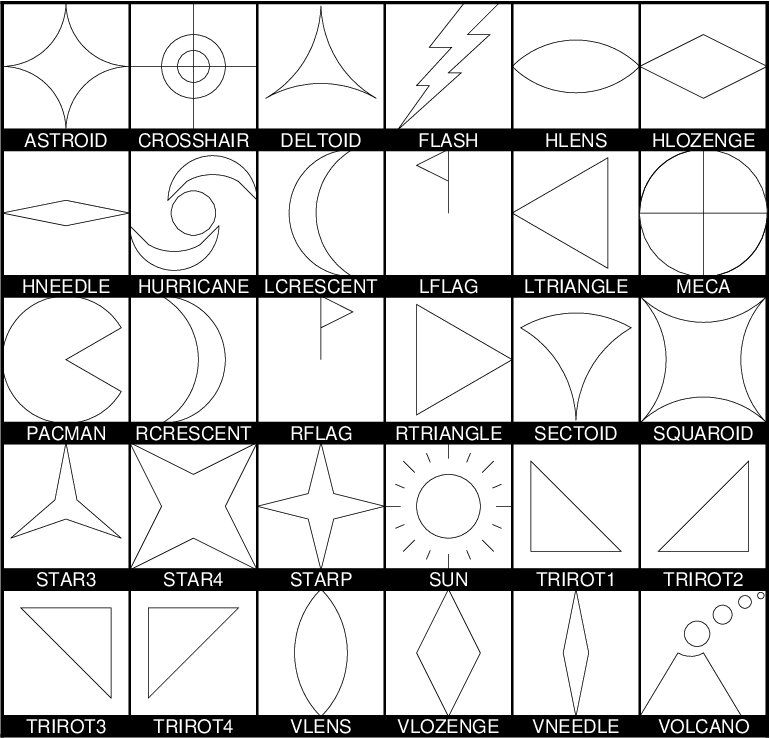
Custom plot symbols supported by GMT. Note that we only show the symbol outline and not any fill. These are all single-parameter symbols. Be aware that some symbols may have a hardwired fill or no-fill component, while others duplicate what is already available as standard built-in symbols.
You may find it convenient to examine some of these and use them as a starting point for your own design; they can be found in GMT’s share/custom directory.
28.2. The macro language
To make your own custom plot symbol, you will need to design your own
*.def files. This section defines the language used to build custom
symbols. You can place these definition files in your current directory
or in your ~/.gmt user directory. When designing the symbol you are working
in a relative coordinate system centered on (0,0). This point will be
mapped to the actual location specified by your data coordinates.
Furthermore, your symbol should be constructed within the domain
\({-\frac{1}{2},+\frac{1}{2},-\frac{1}{2},+\frac{1}{2}}\), resulting
in a 1 by 1 relative canvas area. This 1 x 1 square will be scaled to your
actual symbol size when plotted. However, there are no requirement that
all your design fit inside this domain.
28.2.1. Comment lines
Your definition file may have any number of comment lines, defined to begin with the character #. These are skipped by GMT but provides a mechanism for you to clarify what your symbol does.
28.2.2. Symbol variables
Simple symbols, such as circles and triangles, only take a single parameter: the symbol size, which is either given on the command line (via -Sk) or as part of the input data. However, more complicated symbols that involve angles, or conditional tests, may require more parameters. If your custom symbol requires more than the implicit single size parameter you must include the line
N: n_extra_parameters [types]
before any other macro commands. It is an optional statement in that n_extra_parameters will default to 0 unless explicitly set. By default the extra parameters are considered to be quantities that should be passed directly to the symbol machinery. However, you can use the types argument to specify different types of parameters and thus single out parameters for pre-processing. The available types are
a Geographic azimuth (positive clockwise from north toward east). Parameters identified as azimuth will first be converted to map angle (positive counter-clockwise from horizontal) given the current map projection (or simply via 90-azimuth for Cartesian plots). We ensure the angles fall in the 0-360 range and any macro test can rely on this range.
l Length, i.e., an additional length scale (in cm, inch, or point as per PROJ_LENGTH_UNIT) in addition to the given symbol size.
o Other, i.e., a numerical quantity to be passed to the custom symbol unchanged.
r rotation angles (positive counter-clockwise from horizontal). We ensure the angles fall in the 0-360 range and any macro test can rely on this range.
s String, i.e., a single column of text to be placed by the l command. Use octal \040 to include spaces to ensure the text string remains a single word.
To use the extra parameters in your macro you address them as $1, $2, etc. There is no limit on how many parameters your symbol may use.
28.2.3. Macro commands
The custom symbol language contains commands to rotate the relative coordinate system, draw free-form polygons and lines, change the current fill and/or pen, place text, and include basic geometric symbols as part of the overall design (e.g., circles, triangles, etc.). The available commands are listed in Table custsymb. Note that all angles in the arguments can be provided as variables while the remaining parameters are constants.
| Name | Code | Purpose | Arguments |
|---|---|---|---|
| rotate | R | Rotate the coordinate system | \(\alpha\)[a] |
| moveto | M | Set a new anchor point | \(x_0, y_0\) |
| drawto | D | Draw line from previous point | \(x, y\) |
| arc | A | Append circular arc to existing path | \(x_c, y_c, d, \alpha_1, \alpha_2\) |
| stroke | S | Stroke existing path only | |
| texture | T | Change current pen and fill | |
| star | a | Plot a star | \(x, y\),size |
| circle | c | Plot a circle | \(x, y\),size |
| diamond | d | Plot a diamond | \(x, y\),size |
| ellipse | e | Plot a ellipse | \(x, y, \alpha\),major,minor |
| octagon | g | Plot an octagon | \(x, y\),size |
| hexagon | h | Plot a hexagon | \(x, y\),size |
| invtriangle | i | Plot an inverted triangle | \(x, y\),size |
| rotrectangle | j | Plot an rotated rectangle | \(x, y, \alpha\),width,height |
| letter | l | Plot a letter | \(x, y\),size, string |
| marc | m | Plot a math arc (no heads) | \(x, y, r, \alpha_1, \alpha_2\) |
| pentagon | n | Plot a pentagon | \(x, y\),size |
| plus | + | Plot a plus sign | \(x, y\),size |
| rect | r | Plot a rectangle | \(x, y\), width, height |
| square | s | Plot a square | \(x, y\),size |
| triangle | t | Plot a triangle | \(x, y\),size |
| wedge | w | Plot a wedge | \(x, y, d, \alpha_1, \alpha_2\) |
| cross | x | Plot a cross | \(x, y\),size |
| x-dash | - | Plot a x-dash | \(x, y\),size |
| y-dash | y | Plot a y-dash | \(x, y\),size |
Note for R: if an a is appended to the angle then \(\alpha\) is considered to be a map azimuth; otherwise it is a Cartesian map angle. The a modifier does not apply if the angle is given via a variable, in which case the type of angle has already been specified via N: above and already converged before seen by R.
28.2.4. Symbol fill and outline
Normally, symbols, polygons and lines will be rendered using any fill and outline options you have given on the command line, similarly to how the regular built-in symbols behave. For M, T, and all the lower-case symbol codes you may optionally append specific pens (with -Wpen) and fills (with -Gpen). These options will force the use of these settings and ignore any pens and fills you may or may not have specified on the command line. Passing -G- or -W- means a symbol or polygon will have no fill or outline, respectively, regardless of what your command line settings are. Unlike pen options on the command line, a pen setting inside the macro symbol offers more control. Here, pen width is a dimension and you can specify it in three different ways: (1) Give a fixed pen width with trailing unit (e.g., -W1p,red); we then apply that pen exactly as it is regardless of the size of the symbol, (2) give a normalized pen thickness in the 0-1 range (e.g., -W0.02); at run-time this thickness will be multiplied by the current symbol size to yield the actual pen thickness, and (3) specify a variable pen thickness (e.g., -W$1,blue); we then obtain the actual pen thickness from the data record at run-time. Finally, you may indicate that a symbol or polygon should be filled using the color of the current pen instead of the current fill; do this by specifying -G+p. Likewise, you may indicate that an outline should be drawn with the color of the current fill instead of the current pen; do this by appending +g to your -W setting (which may also indicate pen thickness and texture). E.g., -W1p,-+g would mean “draw the outline with a 1p thick dashed pen but obtain the color from the current fill”.
28.2.5. Symbol substitution
Custom symbols that need to plot any of the standard geometric symbols (i.e., those controlled by a single size) can make the symbol code a variable. By specifying ? instead of the symbol codes a, c, d, g, h, i, n, +, s, t, x, -, or y the actual symbol code is expected to be found at the end of each data record. Such custom symbols must be invoked with -SK rather than -Sk.
28.2.6. Text substitution
Normally, the l macro code will place a hard-wired text string. However, you can also obtain the entire string from your input file via a single symbol variable that must be declared with type s (string). The string read from your input file must be a single word, so if you need to insert spaces you must use the octal \040 code instead. Similarly, to place the dollar sign $ itself you must use octal \044 so as to not confuse the parser with a symbol variable. The string itself, if obtained from the symbol definition file, may contain special codes that will be expanded given information from the current record. You can embed the codes %X or %Y to add the current longitude (or x) and latitude (or y) in your label string. You may also use $n (n is 1, 2, etc.) to embed a numerical symbol variable as text. It will be formatted according to FORMAT_FLOAT_MAP, unless you append the modifiers +X (format as longitude via FORMAT_GEO_MAP), +Y (format as latitude via FORMAT_GEO_MAP), or +T (format as calendar time via FORMAT_DATE_MAP and FORMAT_CLOCK_MAP.
28.2.7. Text alignment and font attributes
Like the Sl symbol in psxy, you can change the current font by appending to l the modifier +ffont [FONT_ANNOT_PRIMARY] and change the text justification by appending the modifier +jjustify [CM]. Note: Here, the font specification will only be considered for the font type and not its size (which is set separately by your size argument) or color and outline (which are set separately by -G and -W arguments). Finally, there are two ways to specify the font size. If a fixed font size is given in points (e.g,, 12p) then the text will be set at that size regardless of the symbol size specified in -S. Without the trailing p we interpret the size as a relative size in the 0-1 range and the actual font size will then scale with the symbol size, just like other symbol items.
28.2.8. Conditional statements
There are two types of conditional statements in the macro language: A simple condition preceding a single command, or a more elaborate if-then-elseif-else construct. In any test you may use one (and only one) of many logical operators, as listed in Table custop.
| Operator | Purpose |
|---|---|
| < | Is left less than right? |
| <= | Is left less than or equal to right? |
| == | Is left equal to right? |
| != | Is left not equal to right? |
| >= | Is left greater than or equal to right? |
| > | Is left greater than right? |
| % | Does left have a remainder with right? |
| !% | Is left an exact multiple of right? |
| <> | Is left within the exclusive range of right? |
| [] | Is left within the inclusive range of right? |
| <] | Is left within the in/ex-clusive range of right? |
| [> | Is left within the ex/in-clusive range of right? |
Above, left refers to one of your variable arguments (e.g., $1, $2) or any constant (e.g. 45) on the left hand side of the operator. On the right hand side of the operator, right is either one of your other variables, or a constant, or a range indicated by two colon-separated constants or variables (e.g., 10:50, $2:60, $3:$4, etc.).
28.2.8.1. Simple conditional test
The simple if-test uses a one-line format, defined as
if left OP right then command
where left must be one of the symbol parameters, specified as $1, $2, $3, etc., or a constant. You must document what these additional parameters control. For example, to plot a small cyan circle at (0.2, 0.3) with diameter 0.4 only if $2 exceeds 45 you would write
if $2 > 45 then 0.2 0.3 0.4 c -Gcyan
Note that this form of the conditional test has no mechanism for an else branch, but this can be accomplished by repeating the test but reversing the logic for the second copy, e.g.,
if $1 > 10 then 0 0 0.5 c -Gred
if $1 <= 10 then 0 0 0.5 c -Gblue
or you may instead consider the complete conditional construct below. Using a comparison between variables is similarly straightforward:
if $2 > $3 then 0.2 0.3 0.4 c -Ggreen
28.2.8.2. Complete conditional test
The complete conditional test uses a multi-line format, such as
The elseif (one or more) and else branches are optional. Note that the syntax is strictly enforced, meaning the opening brace must appear after then with nothing following it, and the closing brace must appear by itself with no other text, and that the elseif and else statements must have both closing and opening braces on the same line (and nothing else). If you need comments please add them as separate lines. You may nest tests as well (up to 10 levels deep), e.g.,
if $1 > 45 then {
        if $2 [> 0:10 then 0 0 0.5 c -Gred
} elseif $1 < 15 then {
        if $2 [> 0:10 then 0 0 0.5 c -Ggreen
} else {
        if $2 [> 10:20 then {
                0 0 M -W1p,blue
                0.3 0.3 D
                S
                0.3 0.3 0.3 c -Gcyan
        }
}
29. Annotation of Contours and “Quoted Lines”
The GMT programs grdcontour (for data given as 2-dimensional grids) and pscontour (for x,y,z tables) allow for contouring of data sets, while psxy and psxyz can plot lines based on x,y- and x,y,z-tables, respectively. In both cases it may be necessary to attach labels to these lines. Clever or optimal placements of labels is a very difficult topic, and GMT provides several algorithms for this placement as well as complete freedom in specifying the attributes of the labels. Because of the richness of these choices we present this Chapter which summarizes the various options and gives several examples of their use.
29.1. Label Placement
While the previous GMT versions 1--3 allowed for a single algorithm that determined where labels would be placed, GMT 4 allows for five different algorithms. Furthermore, a new “symbol” option (-Sq for “quoted line”) has been added to psxy and psxyz and hence the new label placement mechanisms apply to those programs as well. The contouring programs expect the algorithm to be specified as arguments to -G while the line plotting programs expect the same arguments to follow -Sq. The information appended to these options is the same in both cases and is of the form [code]info. The five algorithms correspond to the five codes below (some codes will appear in both upper and lower case; they share the same algorithm but differ in some other ways). In what follows, the phrase “line segment” is taken to mean either a contour or a line to be labeled. The codes are:
- d:
- Full syntax is ddist[c|i|p][/frac]. Place labels according to the distance measured along the projected line on the map. Append the unit you want to measure distances in [Default is taken from PROJ_LENGTH_UNIT]. Starting at the beginning of a line, place labels every dist increment of distance along the line. To ensure that closed lines whose total length is less than dist get annotated, we may append frac which will place the first label at the distance d = dist \(\times\) frac from the start of a closed line (and every dist thereafter). If not given, frac defaults to 0.25.
- D:
- Full syntax is Ddist[d|m|s|e|f|k|M|n][/frac]. This option is similar to d except the original data must be referred to geographic coordinates (and a map projection must have been chosen) and actual Earth [41] surface distances along the lines are considered. Append the unit you want to measure distances in; choose among arc degree, minute, and second, or meter [Default], feet, kilometer, statute Miles, or nautical miles. Other aspects are similar to code d.
- f:
- Full syntax is ffix.txt[/slop[c|i|p]]. Here, an ASCII file fix.txt is given which must contain records whose first two columns hold the coordinates of points along the lines at which locations the labels should be placed. Labels will only be placed if the coordinates match the line coordinates to within a distance of slop (append unit or we use PROJ_LENGTH_UNIT). The default slop is zero, meaning only exact coordinate matches will do.
- l:
- Full syntax is lline1[,line2[, …]]. One or more straight line segments are specified separated by commas, and labels will be placed at the intersections between these lines and our line segments. Each line specification implies a start and stop point, each corresponding to a coordinate pair. These pairs can be regular coordinate pairs (i.e., longitude/latitude separated by a slash), or they can be two-character codes that refer to predetermined points relative to the map region. These codes are taken from the pstext justification keys [L|C|R][B|M|T] so that the first character determines the x-coordinate and the second determines the y-coordinate. In grdcontour, you can also use the two codes Z+ and Z- as shorthands for the location of the grid’s global maximum and minimum, respectively. For example, the line LT/RB is a diagonal from the upper left to the lower right map corner, while Z-/135W/15S is a line from the grid minimum to the point (135ºW, 15ºS).
- L:
- Same as l except we will treat the lines given as great circle start/stop coordinates and fill in the points between before looking for intersections. You must make sure not to give antipodal start and stop coordinates since the great circle path would be undefined.
- n:
- Full syntax is nnumber[/minlength[c|i|p]]. Place number of labels along each line regardless of total line length. The line is divided into number segments and the labels are placed at the centers of these segments. Optionally, you may give a minlength distance to ensure that no labels are placed closer than this distance to its neighbors.
- N:
- Full syntax is Nnumber[/minlength[c|i|p]]. Similar to code n but here labels are placed at the ends of each segment (for number >= 2). A special case arises for number = 1 when a single label will be placed according to the sign of number: -1 places one label justified at the start of the line, while +1 places one label justified at the end of the line.
- s:
- Similar to n but splits input lines into a series of two-point line segments first. The rest of the algorithm them operates on these sets of lines. This code (and S) are specific to quoted lines.
- S:
- Similar to N but with the modification described for s.
- x:
- Full syntax is xcross.d. Here, an ASCII file cross.d is a multi-segment file whose lines will intersect our segment lines; labels will be placed at these intersections.
- X:
- Same as x except we treat the lines given as great circle start/stop coordinates and fill in the points between before looking for intersections.
Only one algorithm can be specified at any given time.
29.2. Label Attributes
Determining where to place labels is half the battle. The other half is to specify exactly what are the attributes of the labels. It turns out that there are quite a few possible attributes that we may want to control, hence understanding how to specify these attributes becomes important. In the contouring programs, one or more attributes may be appended to the -A option using the format +code[args] for each attribute, whereas for the line plotting programs these attributes are appended to the -Sq option following a colon (:) that separates the label codes from the placement algorithm. Several of the attributes do not apply to contours so we start off with listing those that apply universally. These codes are:
- +a:
- Controls the angle of the label relative to the angle of the line. Append n for normal to the line, give a fixed angle measured counter-clockwise relative to the horizontal. or append p for parallel to the line [Default]. If using grdcontour the latter option you may further append u or d to get annotations whose upper edge always face the next higher or lower contour line.
- +c:
- Surrounding each label is an imaginary label “textbox” which defines a region in which no segment lines should be visible. The initial box provides an exact fit to the enclosed text but clearance may be extended in both the horizontal and vertical directions (relative to the label baseline) by the given amounts. If these should be different amounts please separate them by a slash; otherwise the single value applies to both directions. Append the distance units of your choice (c|i|m|p), or give % to indicate that the clearance should be this fixed percentage of the label font size in use. The default is 15%.
- +d:
- Debug mode. This is useful when testing contour placement as it will draw the normally invisible helper lines and points in the label placement algorithms above.
- +e:
- Delayed mode, to delay the plotting of the text as text clipping is set instead.
- +f:
- Specifies the desired label font, including size or color. See pstext for font names or numbers. The default font is given by FONT_ANNOT_PRIMARY.
- +g:
- Selects opaque rather than the default transparent text boxes. You may optionally append the color you want to fill the label boxes; the default is the same as PS_PAGE_COLOR.
- +j:
- Selects the justification of the label relative to the placement points determined above. Normally this is center/mid justified (CM in pstext justification parlance) and this is indeed the default setting. Override by using this option and append another justification key code from [L|C|R][B|M|T]. Note for curved text (+v) only vertical justification will be affected.
- +o:
- Request a rounded, rectangular label box shape; the default is rectangular. This is only manifested if the box is filled or outlined, neither of which is implied by this option alone (see +g and +p). As this option only applies to straight text, it is ignored if +v is given.
- +p:
- Selects the drawing of the label box outline; append your preferred pen unless you want the default GMT pen [0.25p,black].
- +r:
- Do not place labels at points along the line whose local radius of curvature falls below the given threshold value. Append the radius unit of your choice (c|i|p) [Default is 0].
- +u:
- Append the chosen unit to the label. Normally a space will separate the label and the unit. If you want to close this gap, append a unit that begins with a hyphen (-). If you are contouring with grdcontour and you specify this option without appending a unit, the unit will be taken from the z-unit attribute of the grid header.
- +v:
- Place curved labels that follow the wiggles of the line segments. This is especially useful if the labels are long relative to the length-scale of the wiggles. The default places labels on an invisible straight line at the angle determined.
- +w:
- The angle of the line at the point of straight label placement is calculated by a least-squares fit to the width closest points. If not specified, width defaults to 10.
- +=:
- Similar in most regards to +u but applies instead to a label prefix which you must append.
For contours, the label will be the value of the contour (possibly modified by +u or +=). However, for quoted lines other options apply:
- +l:
- Append a fixed label that will be placed at all label locations. If the label contains spaces you must place it inside matching quotes.
- +L:
Append a code flag that will determine the label. Available codes are:
- +Lh:
- Take the label from the current multi-segment header (hence it is assumed that the input line segments are given in the multi-segment file format; if not we pick the single label from the file’s header record). We first scan the header for an embedded -Llabel option; if none is found we instead use the first word following the segment marker [>].
- +Ld:
- Take the Cartesian plot distances along the line as the label; append c|i|p as the unit [Default is PROJ_LENGTH_UNIT]. The label will be formatted according to the FORMAT_FLOAT_OUT string, unless label placement was determined from map distances along the segment lines, in which case we determine the appropriate format from the distance value itself.
- +LD:
- Calculate actual Earth surface distances and use the distance at the label placement point as the label; append d|e|f|k|m|M|n|s to specify the unit [If not given we default to degrees, unless label placement was determined from map distances along the segment lines, in which case we use the same unit specified for that algorithm]. Requires a map projection to be used.
- +Lf:
- Use all text after the 2nd column in the fixed label location file fix.txt as labels. This choice obviously requires the fixed label location algorithm (code f) to be in effect.
- +Ln:
- Use the running number of the current multi-segment as label.
- +LN:
- Use a slash-separated combination of the current file number and the current multi-segment number as label.
- +Lx:
- As h but use the multi-segment headers in the cross.d file instead. This choice obviously requires the crossing segments location algorithm (code x|X) to be in effect.
29.3. Examples of Contour Label Placement
We will demonstrate the use of these options with a few simple examples. First, we will contour a subset of the global geoid data used in Example (1) Contour maps; the region selected encompasses the world’s strongest “geoid dipole”: the Indian Low and the New Guinea High.
29.3.1. Equidistant labels
Our first example uses the default placement algorithm. Because of the size of the map we request contour labels every 1.5 inches along the lines:
gmt pscoast -R50/160/-15/15 -JM5.3i -Gburlywood -Sazure -A500 -K -P > GMT_App_O_1.ps
gmt grdcontour geoid.nc -J -O -B20f10 -BWSne -C10 -A20+f8p -Gd1.5i -S10 -T+lLH >> GMT_App_O_1.ps
As seen in Figure Contour label 1, the contours are placed rather arbitrary. The string of contours for -40 to 60 align well but that is a fortuitous consequence of reaching the 1.5 inch distance from the start at the bottom of the map.
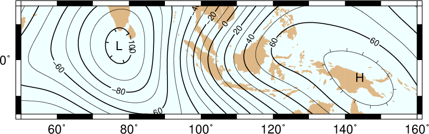
Equidistant contour label placement with -Gd, the only algorithm available in previous GMT versions.
29.3.2. Fixed number of labels
We now exercise the option for specifying exactly how many labels each contour line should have:
gmt pscoast -R50/160/-15/15 -JM5.3i -Gburlywood -Sazure -A500 -K -P > GMT_App_O_2.ps
gmt grdcontour geoid.nc -J -O -B20f10 -BWSne -C10 -A20+f8p -Gn1/1i -S10 -T+lLH >> GMT_App_O_2.ps
By selecting only one label per contour and requiring that labels only be placed on contour lines whose length exceed 1 inch, we achieve the effect shown in Figure Contour label 2.
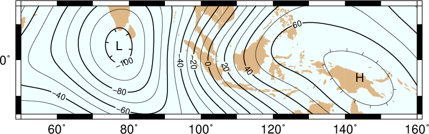
Placing one label per contour that exceed 1 inch in length, centered on the segment with -Gn.
29.3.3. Prescribed label placements
Here, we specify four points where we would like contour labels to be placed. Our points are not exactly on the contour lines so we give a nonzero “slop” to be used in the distance calculations: The point on the contour closest to our fixed points and within the given maximum distance will host the label.
cat << EOF > fix.txt
80      -8.5
55      -7.5
102     0
130     10.5
EOF
gmt pscoast -R50/160/-15/15 -JM5.3i -Gburlywood -Sazure -A500 -K -P > GMT_App_O_3.ps
gmt grdcontour geoid.nc -J -O -B20f10 -BWSne -C10 -A20+d+f8p -Gffix.txt/0.1i -S10 -T+lLH >> GMT_App_O_3.ps
The angle of the label is evaluated from the contour line geometry, and the final result is shown in Figure Contour label 3. To aid in understanding the algorithm we chose to specify “debug” mode (+d) which placed a small circle at each of the fixed points.
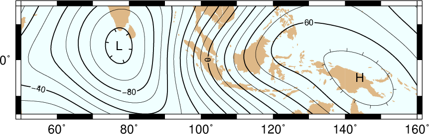
Four labels are positioned on the points along the contours that are closest to the locations given in the file fix.txt in the -Gf option.
29.3.4. Label placement at simple line intersections
Often, it will suffice to place contours at the imaginary intersections between the contour lines and a well-placed straight line segment. The -Gl or -GL algorithms work well in those cases:
gmt pscoast -R50/160/-15/15 -JM5.3i -Gburlywood -Sazure -A500 -K -P > GMT_App_O_4.ps
gmt grdcontour geoid.nc -J -O -B20f10 -BWSne -C10 -A20+d+f8p -GLZ-/Z+ -S10 -T+lLH >> GMT_App_O_4.ps
The obvious choice in this example is to specify a great circle between the high and the low, thus placing all labels between these extrema.
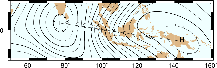
Labels are placed at the intersections between contours and the great circle specified in the -GL option.
The thin debug line in Figure Contour label 4 shows the great circle and the intersections where labels are plotted. Note that any number of such lines could be specified; here we are content with just one.
29.3.5. Label placement at general line intersections
If (1) the number of intersecting straight line segments needed to pick the desired label positions becomes too large to be given conveniently on the command line, or (2) we have another data set or lines whose intersections we wish to use, the general crossing algorithm makes more sense:
gmt pscoast -R50/160/-15/15 -JM5.3i -Gburlywood -Sazure -A500 -K -P > GMT_App_O_5.ps
gmt grdcontour geoid.nc -J -O -B20f10 -BWSne -C10 -A20+d+f8p -GXcross.txt -S10 -T+lLH >> GMT_App_O_5.ps
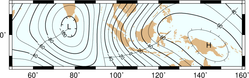
Labels are placed at the intersections between contours and the multi-segment lines specified in the -GX option.
In this case, we have created three strands of lines whose intersections with the contours define the label placements, presented in Figure Contour label 5.
29.4. Examples of Label Attributes
We will now demonstrate some of the ways to play with the label attributes. To do so we will use psxy on a great-circle line connecting the geoid extrema, along which we have sampled the ETOPO5 relief data set. The file thus contains lon, lat, dist, geoid, relief, with distances in km.
29.4.1. Label placement by along-track distances, 1
This example will change the orientation of labels from along-track to across-track, and surrounds the labels with an opaque, outlined text box so that the label is more readable. We choose the place the labels every 1000 km along the line and use that distance as the label. The labels are placed normal to the line:
gmt pscoast -R50/160/-15/15 -JM5.3i -Gburlywood -Sazure -A500 -K -P > GMT_App_O_6.ps
gmt grdcontour geoid.nc -J -O -K -B20f10 -BWSne -C10 -A20+d+f8p -Gl50/10S/160/10S -S10 \
-T+l"-+" >> GMT_App_O_6.ps
gmt psxy -R -J -O -SqD1000k:+g+LD+an+p -Wthick transect.txt >> GMT_App_O_6.ps
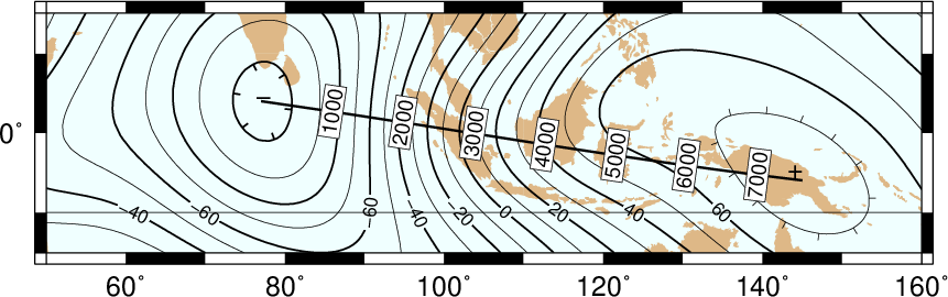
Labels attributes are controlled with the arguments to the -Sq option.
The composite illustration in Figure Contour label 6 shows the new effects. Note that the line connecting the extrema does not end exactly at the ‘-‘ and ‘+’ symbols. This is because the placements of those symbols are based on the mean coordinates of the contour and not the locations of the (local or global) extrema.
29.4.2. Label placement by along-track distances, 2
A small variation on this theme is to place the labels parallel to the line, use spherical degrees for placement, append the degree symbol as a unit for the labels, choose a rounded rectangular text box, and inverse-video the label:
gmt pscoast -R50/160/-15/15 -JM5.3i -Gburlywood -Sazure -A500 -K -P > GMT_App_O_7.ps
gmt grdcontour geoid.nc -J -O -K -B20f10 -BWSne -C10 -A20+d+u" m"+f8p -Gl50/10S/160/10S -S10 \
-T+l"-+" >> GMT_App_O_7.ps
gmt psxy -R -J -O -SqD15d:+gblack+fwhite+Ld+o+u\\260 -Wthick transect.txt >> GMT_App_O_7.ps
The output is presented as Figure Contour label 7.
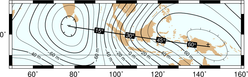
Another label attribute example.
29.4.3. Using a different data set for labels
In the next example we will use the bathymetry values along the transect as our label, with placement determined by the distance along track. We choose to place labels every 1500 km. To do this we need to pull out those records whose distances are multiples of 1500 km and create a “fixed points” file that can be used to place labels and specify the labels. This is done with awk.
gmt convert -i0,1,4 -Em150 transect.txt | $AWK '{print $1,$2,int($3)}' > fix2.txt
gmt pscoast -R50/160/-15/15 -JM5.3i -Gburlywood -Sazure -A500 -K -P > GMT_App_O_8.ps
gmt grdcontour geoid.nc -J -O -K -B20f10 -BWSne -C10 -A20+d+u" m"+f8p -Gl50/10S/160/10S \
               -S10 -T+l"-+" >> GMT_App_O_8.ps
gmt psxy -R -J -O -Sqffix2.txt:+g+an+p+Lf+u" m"+f8p -Wthick transect.txt >> GMT_App_O_8.ps
The output is presented as Figure Contour label 8.
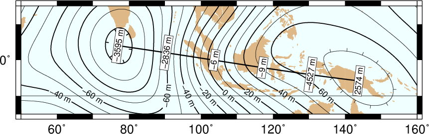
Labels based on another data set (here bathymetry) while the placement is based on distances.
29.5. Putting it all together
Finally, we will make a more complex composite illustration that uses several of the label placement and label attribute settings discussed in the previous sections. We make a map showing the tsunami travel times (in hours) from a hypothetical catastrophic landslide in the Canary Islands [42]. We lay down a color map based on the travel times and the shape of the seafloor, and travel time contours with curved labels as well as a few quoted lines. The final script is
R=-R-85/5/10/55
gmt grdgradient topo5.nc -Nt1 -A45 -Gtopo5_int.nc
gmt set FORMAT_GEO_MAP ddd:mm:ssF FONT_ANNOT_PRIMARY +9p FONT_TITLE 22p
gmt project -E-74/41 -C-17/28 -G10 -Q > great_NY_Canaries.txt
gmt project -E-74/41 -C2.33/48.87 -G100 -Q > great_NY_Paris.txt
km=`echo -17 28 | gmt mapproject -G-74/41/k -fg --FORMAT_FLOAT_OUT=%.0f -o2`
cat << EOF > ttt.cpt
0  lightred        3       lightred
3  lightyellow     6       lightyellow
6  lightgreen      100     lightgreen
EOF
gmt grdimage ttt_atl.nc -Itopo5_int.nc -Cttt.cpt $R -JM5.3i -P -K -nc+t1 > GMT_App_O_9.ps
gmt grdcontour ttt_atl.nc -R -J -O -K -C0.5 -A1+u" hour"+v+f8p,Bookman-Demi \
               -GL80W/31N/17W/26N,17W/28N/17W/50N -S2 >> GMT_App_O_9.ps
gmt psxy -R -J -Wfatter,white great_NY_Canaries.txt -O -K  >> GMT_App_O_9.ps
gmt pscoast -R -J -B20f5 -BWSne+t"Tsunami travel times from the Canaries" -N1/thick -O -K \
            -Glightgray -Wfaint -A500 >> GMT_App_O_9.ps
gmt convert great_NY_*.txt -E | gmt psxy -R -J -O -K -Sa0.15i -Gred -Wthin >> GMT_App_O_9.ps
gmt psxy -R -J -Wthick great_NY_Canaries.txt -O -K \
         -Sqn1:+f8p,Times-Italic+l"Distance Canaries to New York = $km km"+ap+v >> GMT_App_O_9.ps
gmt psxy -R -J great_NY_Paris.txt -O -K -Sc0.08c -Gblack >> GMT_App_O_9.ps
gmt psxy -R -J -Wthinner great_NY_Paris.txt -SqD1000k:+an+o+gblue+LDk+f7p,Helvetica-Bold,white \
         -O -K >> GMT_App_O_9.ps
cat << EOF | gmt pstext -R -J -O -K -Gwhite -Wthin -Dj0.1i/0.1i -F+f8p,Bookman-Demi+j \
                        >> GMT_App_O_9.ps
74W        41N     RT      New York
2.33E      48.87N  CT      Paris
17W        28N     CT      Canaries
EOF
gmt psxy -R -J -O -T >> GMT_App_O_9.ps
with the complete illustration presented as Figure Contour label 9.
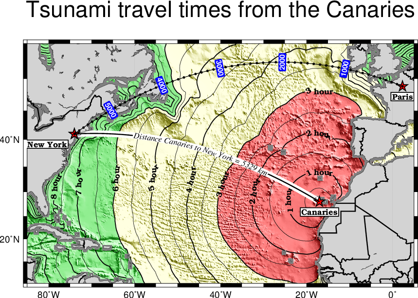
Tsunami travel times from the Canary Islands to places in the Atlantic, in particular New York. Should a catastrophic landslide occur it is possible that New York will experience a large tsunami about 8 hours after the event.
30. Special Operations
30.1. Running GMT in isolation mode
In Chapter General features it is described how GMT creates several (temporary) files to communicate between the different commands that make up the script that finally creates a plot. Among those files are:
- gmt.conf This file covers about 150 different settings that influence the
- layout of your plot, from font sizes to tick lengths and date formats (See Section GMT defaults). Those settings can be altered by editing the file, or by running the gmtset command. A problem may arise when those settings are changed half-way through the script: the next time you run the script it will start with the modified settings and hence might alter your scripts results. It is therefore often necessary to revert to the original
gmt.conffile. Isolation mode avoids that issue.- gmt.history This file is created to communicate the command line history from
- one command to the next (Section Command line history) so that shorthands like -R or -J can be used once it has been set in a previous GMT command. The existence of this file makes if impossible to run two GMT scripts simultaneously in the same directory, since those
gmt.historyfiles may clash (contain different histories) and adversely affect the results of both scripts.
A cure to all these woes is the isolation mode introduced in
GMT version 4.2.2. This mode allows you to run a GMT script without
leaving any traces other than the resulting PostScript or data files,
and not altering the gmt.conf or gmt.history files. Those files will be placed in a temporary
directory instead. And if properly set up, this temporary directory will
only be used by a single script, even if another GMT script is running
simultaneously. This also provides the opportunity to create any other
temporary files that the script might create in the same directory.
The example below shows how isolation mode works.
ps=GMT_App_P_1.ps

# Create a temporary directory. $GMT_TMPDIR will be set to its pathname.
# XXXXXX is replaced by a unique random combination of characters.
export GMT_TMPDIR=`mktemp -d /tmp/gmt.XXXXXX`

# These settings will be local to this script only since it writes to
# $GMT_TMPDIR/gmt.conf
gmt set COLOR_MODEL rgb FONT_ANNOT_PRIMARY 14p

# Make grid file and color map in temporary directory
gmt grdmath -Rd -I1 Y = $GMT_TMPDIR/lat.nc
gmt makecpt -Crainbow -T-90/90/180 -Z > $GMT_TMPDIR/lat.cpt

# The gmt grdimage command creates the history file $GMT_TMPDIR/gmt.history
gmt grdimage $GMT_TMPDIR/lat.nc -JK6.5i -C$GMT_TMPDIR/lat.cpt -P -K -nl > $ps
gmt pscoast -R -J -O -Dc -A5000 -Gwhite -Bx60g30 -By30g30 >> $ps

# Clean up all temporary files and the temporary directory
rm -rf $GMT_TMPDIR
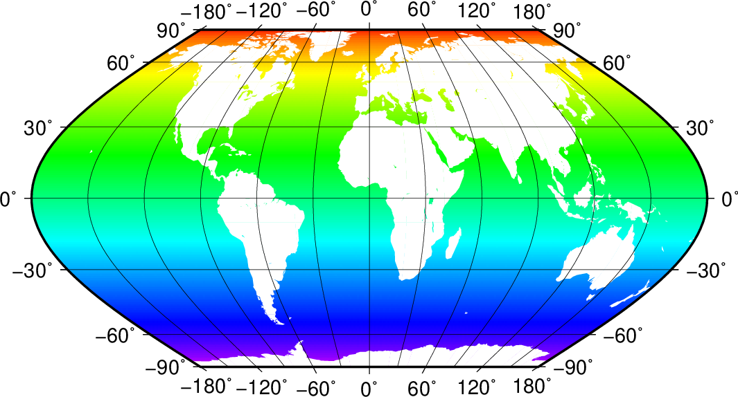
Example created in isolation mode
The files gmt.conf and gmt.history are automatically created in the temporary directory
$GMT_TMPDIR. The script is also adjusted such that the temporary grid file lat.nc and colormap
lat.cpt are created in that directory as well. To make things even more easy,
GMT now provides a set of handy shell functions in gmt_shell_functions.sh:
simply include that file in the script and the creation and the removal
of the temporary directory is reduced to the single commands gmt_init_tmpdir and
gmt_remove_tmpdir, respectively.
31. The GMT Vector Data Format for OGR Compatibility
31.1. Background
The National Institute for Water and Atmospheric Research (NIWA) in New Zealand has funded the implementation of a GMT driver (read and write) for the OGR package. OGR is an Open Source toolkit for accessing or reformatting vector (spatial) data stored in a variety of formats and is part of the. The intention was to enable the easy rendering (using GMT) of spatial data held in non-GMT formats, and the export of vector data (e.g., contours) created by GMT for use with other GIS and mapping packages. While ogr2ogr has had the capability to write this new format since 2009, GMT 4 did not have the capability to use the extra information.
GMT 5 now allows for more advanced vector data, including donut polygons (polygons with holes) and aspatial attribute data. At the same time, the spatial data implementation will not disrupt older GMT 4 programs since all the new information are written via comments.
The identification of spatial feature types in GMT files generally follows the technical description, (which is largely consistent with the OGC SFS specification). This specification provides for non-topological point, line and polygon (area) features, as well as multipoint, multiline and multipolygon features, and was written by Brent Wood based on input from Paul Wessel and others on the GMT team.
31.2. The OGR/GMT format
Several key properties of the OGR/GMT format is summarized below:
- All new data fields are stored as comment lines, i.e., in lines starting with a “#”. OGR/GMT files are therefore compatible with GMT 4 binaries, which will simply ignore this new information.
- To be consistent with current practice in GMT, data fields are represented as whitespace-separated strings within the comments, each identified by the “@” character as a prefix, followed by a single character identifying the content of the field. To avoid confusion between words and strings, the word (field) separator within strings will be the “|” (pipe or vertical bar) character.
- Standard UNIX “" escaping is used, such as \n for newline in a string.
- All new data are stored before the spatial data (coordinates) in the file, so when any GMT 5 program is processing the coordinate data for a feature, it will already have parsed any non-spatial information for each feature, which may impact on how the spatial data is treated (e.g., utilizing the aspatial attribute data for a feature to control symbology).
- The first comment line must specify the version of the OGR/GMT data format, to allow for future changes or enhancements to be supported by future GMT programs. This document describes v1.0.
- For consistency with other GIS formats (such as shapefiles) the OGR/GMT format explicitly contains a field specifying whether the features are points, linestrings or polygons, or the “multi” versions of these. (Other shapefile feature types will not be supported at this stage). At present, GMT programs are informed of this via command line parameters. This will now be explicit in the data file, but does not preclude command line switches setting symbologies for plotting polygons as lines (perimeters) or with fills, as is currently the practice.
- Note that what is currently called a “multiline” (multi-segment) file in GMT parlance is generally a set of “lines” in shapefile/OGR usage. A multiline in this context is a single feature comprising multiple lines. For example, all the transects from a particular survey may be stored as lines, each with it’s own attribute set, such as transect number, date/time, etc. They may also be stored as a single multiline feature with one attribute set, such as trip ID. This difference is explicitly stored in the data in OGR/shapefiles, but currently specified only on the command line in GMT. This applies also to points and polygons. The GMT equivalent to {multipoint, multiline, multipolygon} datatypes is multiple GMT files, each comprising a single {multipoint, multiline, multipolygon} feature.
- The new GMT vector data files includes a header comment specifying the type of spatial features it contains, as well as the description of the aspatial attribute data to be associated with each feature. Unlike the shapefile format, which stores the spatial and aspatial attribute data in separate files, the GMT format will store all data in a single file.
- All the features in a GMT file must be of the same type.
31.3. OGR/GMT Metadata
Several pieces of metadata information must be present in the header of the OGR/GMT file, followed by both spatial and aspatial data. In this section we look at the metadata.
31.3.1. Format version
The comment header line will include a version identifier providing for possible different versions in future. It is indicated by the @V sequence.
| Code | Argument | Description |
|---|---|---|
| V | GMT1.0 | Data in this file is stored using v1.0 of the OGR/GMT data format |
An OGR/GMT file must therefore begin with the line
# @VGMT1.0
Parsing of the OGR/GMT format is only activated if the version code-sequence has been found.
31.3.2. Geometry types
The words and characters used to specify the geometry type (preceded by the @G code sequence on the header comment line), are listed in Table geometries.
| Code | Geometry | Description |
|---|---|---|
| G | POINT | File with point features |
| (Each point will have it’s own attribute/header line preceding the point coordinates) | ||
| G | MULTIPOINT | File with a single multipoint feature |
| (All the point features are a single multipoint, with the same attribute/header | ||
| information) | ||
| G | LINESTRING | File with features comprising multiple single lines |
| (Effectively the current GMT multiline file, each line feature will have it’s own | ||
| attribute and header data) | ||
| G | MULTILINESTRING | File with features comprising a multiline |
| (All the line features in the file are a single multiline feature, only one attribute | ||
| and header which applies to all the lines) | ||
| G | POLYGON | File with one or more polygons |
| (Similar to a line file, except the features are closed polygons) | ||
| G | MULTIPOLYGON | File with a single multipolygon |
| (Similar to a GMT multiline file, except the feature is a closed multipolygon) |
An example GMT polygon file header using this specification (in format 1.0) is
# @VGMT1.0 @GPOLYGON
31.3.3. Domain and map projections
The new format will also support region and projection information. The region will be stored in GMT -R format (i.e., -RW/E/S/N, where the W/E/S/N values represent the extent of features); the @R code sequence marks the domain information. A sample region header is:
# @R150/190/-45/-54
Projection information will be represented as four optional strings, prefixed by @J (J being the GMT character for projection information. The @J code will be followed by a character identifying the format, as shown in Table projectspec.
| Code | Projection Specification |
|---|---|
| @Je | EPSG code for the projection |
| @Jg | A string representing the projection parameters as used by GMT |
| @Jp | A string comprising the Proj.4 parameters representing the projection parameters |
| @Jw | A string comprising the OGR WKT (well known text) representation of the projection parameters |
Sample projection strings are:
# @Je4326 @JgX @Jp"+proj=longlat +ellps=WGS84+datum=WGS84 +no_defs"
# @Jw"GEOGCS[\"WGS84\",DATUM[\"WGS_1984\",SPHEROID\"WGS84\",6378137,\
298.257223563,AUTHORITY[\"EPSG\",\"7030\"]],TOWGS84[0,0,0,0,0,0,0],
AUTHORITY[\"EPSG\",\"6326\"]],PRIMEM[\"Greenwich\",0,\
AUTHORITY[\"EPSG\",\"8901\"]],UNIT[\"degree\",0.01745329251994328,\
AUTHORITY[\"EPSG\",\"9122\"]],AUTHORITY[\"EPSG\",\"4326\"]]"
Note that an OGR-generated file will not have a @Jg string, as OGR does not have any knowledge of the GMT projection specification format. GMT supports at least one of the other formats to provide interoperability with other Open Source related GIS software packages. One relatively simple approach, (with some limitations), would be a lookup table matching EPSG codes to GMT strings.
31.3.4. Declaration of aspatial fields
The string describing the aspatial field names associated with the features is flagged by the @N prefix.
| Code | Argument | Description |
|---|---|---|
| N | word|word|word | A “|” -separated string of names of the attribute field names |
Any name containing a space must be quoted. The @N selection must be combined with a matching string specifying the data type for each of the named fields, using the @T prefix.
| Code | Argument | Description |
|---|---|---|
| T | word|word|word | A “|” -separated string of the attribute field data types |
Available datatypes should largely follow the shapefile (DB3) specification, including string, integer, double, datetime, and logical (boolean). In OGR/GMT vector files, they will be stored as appropriately formatted text strings.
An example header record containing all these is
# @VGMT1.0 @GPOLYGON @Nname|depth|id @Tstring|double|integer
31.4. OGR/GMT Data
All generic fields must be at the start of the file before any feature-specific content (feature attribute data follow the metadata, as do the feature coordinates, separated by a comment line comprising “# FEATURE_DATA”. Provided each string is formatted as specified, and occurs on a line prefixed with “#” (i.e., is a comment), the format is free form, in that as many comment lines as desired may be used, with one or more parameter strings in any order in any line. E.g., one parameter per line, or all parameters on one line.
31.4.1. Embedding aspatial data
Following this header line is the data itself, both aspatial and spatial. For line and polygon (including multiline and multipolygon) data, features are separated using a predefined character, by default “>”. For point (and multipoint) data, no such separator is required. The comment line containing the aspatial data for each feature will immediately precede the coordinate line(s). Thus in the case of lines and polygons, it will immediately follow the “>” line. The data line will be a comment flag (“#”) followed by @D, followed by a string of “|”-separated words comprising the data fields defined in the header record.
To allow for names and values containing spaces, such string items among the @N or @D specifiers must be enclosed in double quotes. (Where double quotes or pipe characters are included in the string, they must be escaped using “"). Where any data values are null, they will be represented as no characters between the field separator, (e.g., #@D|||). A Sample header and corresponding data line for points are
# @VGMT1.0 @GPOINT @Nname|depth|id @Tstring|double|integer
# @D"Point 1"|-34.5|1
while for a polygon it may look like
# @VGMT1.0 @GPOLYGON @Nname|depth|id @Tstring|double|integer
>
# @D"Area 1"|-34.5|1
31.4.2. Polygon topologies
New to GMT is the concept of polygon holes. Most other formats do support this structure, so that a polygon is specified as a sequence of point defining the perimeter, optionally followed by similar coordinate sequences defining any holes (the “donut” polygon concept).
To implement this in a way which is compatible with previous GMT versions, each polygon feature must be able to be identified as the outer perimeter, or an inner ring (hole). This is done using a @P or @H on the data comment preceding the polygon coordinates. The @P specifies a new feature boundary (perimeter), any following @H polygons are holes, and must be within the preceding @P polygon (as described in the shapefile specification). Any @H polygons will NOT have any @D values, as the aspatial attribute data pertain to the entire feature, the @H polygons are not new polygons, but are merely a continuation of the definition of the same feature.
31.5. Examples
Sample point, line and polygon files are (the new data structures are in lines starting with “#” in strings prefixed with “@”). Here is a typical point file:
# @VGMT1.0 @GPOINT @Nname|depth|id
# @Tstring|double|integer
# @R178.43/178.5/-57.98/-34.5
# @Je4326
# @Jp"+proj=longlat +ellps=WGS84 +datum=WGS84+no_defs"
# FEATURE_DATA
# @D"point 1"|-34.5|1
178.5 -45.7
# @D"Point 2"|-57.98|2
178.43 -46.8
...
Next is an example of a line file:
# @VGMT1.0 @GLINESTRING @Nname|depth|id
# @Tstring|double|integer
# @R178.1/178.6/-48.7/-45.6
# @Jp"+proj=longlat +ellps=WGS84 +datum=WGS84+no_defs"
# FEATURE_DATA
> -W0.25p
# @D"Line 1"|-50|1
178.5 -45.7
178.6 -48.2
178.4 -48.7
178.1 -45.6
> -W0.25p
# @D"Line 2"|-57.98|$
178.43 -46.8
...
Finally we show an example of a polygon file:
# @VGMT1.0 @GPOLYGON @N"Polygon name"|substrate|id @Tstring|string|integer
# @R178.1/178.6/-48.7/-45.6
# @Jj@Jp"+proj=longlat +ellps=WGS84 +datum=WGS84+no_defs"
# FEATURE_DATA
> -Gblue -W0.25p
# @P
# @D"Area 1"|finesand|1
178.1 -45.6
178.1 -48.2
178.5 -48.2
178.5 -45.6
178.1 -45.6
>
# @H
# First hole in the preceding perimeter, so is technically still
# part of the same geometry, despite the preceding > character.
# No attribute data is provided, as this is inherited.
178.2 -45.4
178.2 -46.5
178.4 -46.5
178.4 -45.4
178.2 -45.4
>
# @P
...
| [1] | Version 1.0 was then informally released at the Lamont-Doherty Earth Observatory. |
| [2] | See GNU Lesser General Public License (http://www.gnu.org/copyleft/gpl.html) for terms on redistribution and modifications. |
| [3] | The tools can also be installed on other platforms (see Chapter GMT on non-UNIX Platforms). |
| [5] | Programs now also allow for fast, binary multicolumn file i/o. |
| [6] | While the netCDF format is the default, many other formats are also possible. |
| [7] | Vicenty, T. (1975), Direct and inverse solutions of geodesics on the ellipsoid with application of nested equations, Surv. Rev., XXII(176), 88--93. |
| [8] | PostScript definition. In the typesetting industry a slightly different definition of point (1/72.27 inch) is used, presumably to cause needless trouble. |
| [9] | Choose between SI and US default units by modifying in the GMT share directory. |
| [10] | To remain backwards compatible with GMT 4 we will also look for but only if cannot be found. |
| [11] | The Gregorian Calendar is a revision of the Julian Calendar which was instituted in a papal bull by Pope Gregory XIII in 1582. The reason for the calendar change was to correct for drift in the dates of significant religious observations (primarily Easter) and to prevent further drift in the dates. The important effects of the change were (a) Drop 10 days from October 1582 to realign the Vernal Equinox with 21 March, (b) change leap year selection so that not all years ending in “00” are leap years, and (c) change the beginning of the year to 1 January from 25 March. Adoption of the new calendar was essentially immediate within Catholic countries. In the Protestant countries, where papal authority was neither recognized not appreciated, adoption came more slowly. England finally adopted the new calendar in 1752, with eleven days removed from September. The additional day came because the old and new calendars disagreed on whether 1700 was a leap year, so the Julian calendar had to be adjusted by one more day. |
| [12] | While UTM coordinates clearly refer to points on the Earth, in this context they are considered “other”. Thus, when we refer to “geographical” coordinates herein we imply longitude, latitude. |
| [13] | Please consult the man page for printf or any book on C. |
| [14] | For historical reasons, the GMT default is Landscape; see gmt.conf to change this. |
| [15] | Ensures that boundary annotations do not fall off the page. |
| [16] | To keep PostScript files small, such comments are by default turned off; see PS_COMMENTS to enable them. |
| [17] | For an overview of color systems such as HSV, see Chapter Color Space: The Final Frontier. |
| [18] |
|
| [19] | Requires building GMT with GDAL. |
| [20] | Snyder, J. P., 1987, Map Projections A Working Manual, U.S. Geological Survey Prof. Paper 1395. |
| [21] | This is, however, not the shortest distance. It is given by the great circle connecting the two points. |
| [22] | Robinson provided a table of y-coordinates for latitudes every 5. To project values for intermediate latitudes one must interpolate the table. Different interpolants may result in slightly different maps. GMT uses the interpolant selected by the parameter GMT_INTERPOLANT in the file. |
| [23] | (1, 2) These data are available on CD-ROM from NGDC (http://www.ngdc.noaa.gov/). |
| [24] | See http://topex.ucsd.edu/marine_grav/mar_grav.html. |
| [25] | Pedants who wish to argue about the “other” arc going the long way should consider using it. |
| [26] | While Quicktime is free you must upgrade to QuickTime Pro (USD 30) to use the authoring functions. |
| [27] | QuickTime Pro can do this, as can most video-editing programs. |
| [28] | For data bases, see http://topex.ucsd.edu/marine_grav/mar_grav.html. |
| [29] | The ASCII MGD77 data are available on CD-ROM from NGDC (http://www.ngdc.noaa.gov/). |
| [30] | Okabe, M., 1979, Analytical expressions for gravity anomalies due to polyhedral bodies and translation into magnetic anomalies, Geophysics, 44, 730--741. |
| [31] | Talwani, M., J. L. Worzel, and M. Landisman (1959), Rapid gravity computations for two-dimensional bodies with application to the Mendocino submarine fracture zone, J. Geophys. Res., 64, 49-–59. |
| [32] | Talwani, M., and M. Ewing (1960), Rapid computation of gravitational attraction of three-dimensional bodies of arbitrary shape, Geophysics, 25, 203--225. |
| [33] | Timothy J. Henstock, University of Southampton |
| [34] | If you chose SI units during the installation then the default encoding is ISOLatin1+, otherwise it is Standard+. |
| [35] | R. Bracewell, The Fourier Transform and its Applications, McGraw-Hill, London, 444 p., 1965. |
| [36] | National Geophysical Data Center, Boulder, Colorado |
| [37] | Douglas, D.H., and T. K. Peucker, 1973, Algorithms for the reduction of the number of points required to represent a digitized line or its caricature, Canadian Cartographer, 10, 112--122. |
| [38] | The full and high resolution files are in separate archives because of their size. Not all users may need these files as the intermediate data set is better than the data provided with version 2.2.4. |
| [39] | If you need complete polygons in a simpler format, see the article on GSHHG (Wessel, P., and W. H. F. Smith, 1996, A Global, self-consistent, hierarchical, high-resolution shoreline database, J. Geophys. Res. 101, 8741--8743). |
| [40] | The 3rd palette is called categorical and produces a set of colors suitable for categorical plots. |
| [41] | or whatever planet we are dealing with. |
| [42] | Travel times were calculated using Geoware’s travel time calculator, ttt; see http://www.geoware-online.com/. |