(3) Spectral estimation and xy-plots
In this example we will show how to use the GMT programs
fitcircle, project,
sample1d, spectrum1d,
and plot. Suppose you have (lon, lat,
gravity) along a satellite track in a file called sat.xyg, and (lon, lat,
gravity) along a ship track in a file called ship.xyg. You want to make a
cross-spectral analysis of these data. First, you will have to get the
two data sets into equidistantly sampled time-series form. To do this,
it will be convenient to project these along the great circle that best
fits the sat track. We must use
fitcircle to find this great circle
and choose the L2 estimates of best pole. We project the data
using project to find out what their
ranges are in the projected coordinate. The
gmtinfo utility will report the minimum
and maximum values for multi-column ASCII tables. Use this information
to select the range of the projected distance coordinate they have in
common. The script computes the common range. We can then resample the projected data, and carry
out the cross-spectral calculations, assuming that the ship is the input
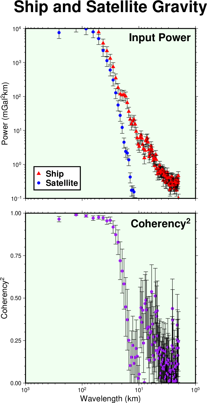
and the satellite is the output data. The final plot example_03.ps shows the ship and sat power
in one diagram and the coherency on another diagram, both on the same
page, with an auto-generated legend. Thus, the complete automated script reads:
#!/usr/bin/env bash
#		GMT EXAMPLE 03
#
# Purpose:	Resample track data, do spectral analysis, and plot
# GMT modules:	filter1d, fitcircle, gmtconvert, gmtinfo, project, sample1d
# 		spectrum1d, plot, subplot, legend, math
# Unix progs:	rm
#
# This example begins with data files "ship_03.txt" and "sat_03.txt" which
# are measurements of a quantity "g" (a "gravity anomaly" which is an
# anomalous increase or decrease in the magnitude of the acceleration
# of gravity at sea level).  g is measured at a sequence of points "x,y"
# which in this case are "longitude,latitude".  The "sat_03.txt" data were
# obtained by a satellite and the sequence of points lies almost along
# a great circle.  The "ship_03.txt" data were obtained by a ship which
# tried to follow the satellite's path but deviated from it in places.
# Thus the two data sets are not measured at the same of points,
# and we use various GMT tools to facilitate their comparison.
#

gmt begin ex03
	gmt set GMT_FFT kiss
	# First, we use "gmt fitcircle" to find the parameters of a great circle
	# most closely fitting the x,y points in "sat_03.txt":
	cpos=$(gmt fitcircle @sat_03.txt -L2 -Fm --IO_COL_SEPARATOR=/)
	ppos=$(gmt fitcircle @sat_03.txt -L2 -Fn --IO_COL_SEPARATOR=/)
	# Now we use "gmt project" to project the data in both sat_03.txt and ship_03.txt
	# into data.pg, where g is the same and p is the oblique longitude around
	# the great circle.  We use -Q to get the p distance in kilometers, and -S
	# to sort the output into increasing p values.
	gmt project  @sat_03.txt -C$cpos -T$ppos -S -Fpz -Q > sat.pg
	gmt project @ship_03.txt -C$cpos -T$ppos -S -Fpz -Q > ship.pg
	bounds=$(gmt info ship.pg sat.pg -I1 -Af -L -C -i0  --IO_COL_SEPARATOR=/)
	# Now we can use $bounds in gmt math to make a sampling points file for gmt sample1d:
	gmt math -T$bounds/1 -N1/0 T = samp.x
	# Now we can resample the gmt projected satellite data:
	gmt sample1d sat.pg -Tsamp.x > samp_sat.pg
	# For reasons above, we use gmt filter1d to pre-treat the ship data.  We also need to sample
	# it because of the gaps > 1 km we found.  So we use gmt filter1d | gmt sample1d.  We also
	# use the -E on gmt filter1d to use the data all the way out to bounds :
	gmt filter1d ship.pg -Fm1 -T$bounds/1 -E | gmt sample1d -Tsamp.x > samp_ship.pg
	# Now to do the cross-spectra, assuming that the ship is the input and the sat is the output
	# data, we do this:
	gmt convert -A samp_ship.pg samp_sat.pg -o1,3 | gmt spectrum1d -S256 -D1 -W -C -T
	# Time to plot spectra, use -l to build a legend
	gmt set FONT_TAG 18p,Helvetica-Bold
	gmt subplot begin 2x1 -M0.3c -Scb+l"Wavelength (km)" -T"Ship and Satellite Gravity" -Fs10c -A+jTR+o8p -BWeSn+g240/255/240
		gmt subplot set 0,0 -A"Input Power"
		gmt plot spectrum.xpower -JX-?l/?l -Bxa1f3p -Bya1f3p+l"Power (mGal@+2@+km)" -Gred -ST5p -R1/1000/0.1/10000 -Ey+p0.5p -lShip
		gmt plot spectrum.ypower -Gblue -Sc5p -Ey+p0.5p -lSatellite
		gmt legend -DjBL+o0.5c -F+gwhite+pthicker --FONT_ANNOT_PRIMARY=14p,Helvetica-Bold
		gmt subplot set 1,0 -A"Coherency@+2@+"
		gmt plot spectrum.coh -JX-?l/? -Bxa1f3p -Bya0.25f0.05+l"Coherency@+2@+" -R1/1000/0/1 -Sc5p -Gpurple -Ey+p0.5p
	gmt subplot end
gmt end show
rm -f samp* *.pg spectrum.*
The final illustration shows that the ship gravity anomalies have more power than altimetry derived gravity for short wavelengths and that the coherency between the two signals improves dramatically for wavelengths > 20 km.
Spectral estimation and x=y-plots.