17. Of Colors and Color Legends
17.1. Built-in color palette tables (CPT)
Figures CPTs a, b, c and d show the built-in color palettes, stored in so-called CPTs. The programs makecpt and grd2cpt are used to access these master CPTs and translate/scale them to fit the user’s range of z-values. The top half of the color bars in the Figure shows the original color scale, which can be either discrete or continuous, though some (like globe) are a mix of the two. The bottom half the color bar are built by using makecpt -T-1/1/0.25, thus splitting the color scale into 8 discrete colors. Black and white triangles indicate which tables have hard or soft hinges, respectively. Some CPTs have a default z-range while others are dynamic. Default ranges, if available, are indicated on the top-right of the scales.
The color maps are subdivided into a number of sections relating to their source. This avoids name clashes and improves recognition of the color maps as well as their authors:
gmt: color maps originally produced by the GMT authors and available in GMT for a long time;
SCM: Scientific Colour Maps by Fabio Crameri;
cmocean: ocean color maps by Kirsten Thyng;
cpt-city: color maps ported from the cpt-city archive;
google: color maps promoted by Google;
matlab: a selection of color maps supported by Matlab;
matplotlib: popular color maps from the matplotlib selection;
panoply: color maps from the Panoply application.
Color maps can be selected in various of the GMT tools using -C[section/] cpt, where cpt is the color map name (without the .cpt extension) and section is one of the color map sections mentioned above. If section is omitted, the first matching cpt in those sections is used. Thus -Cglobe and -Cgmt/globe are equivalent.
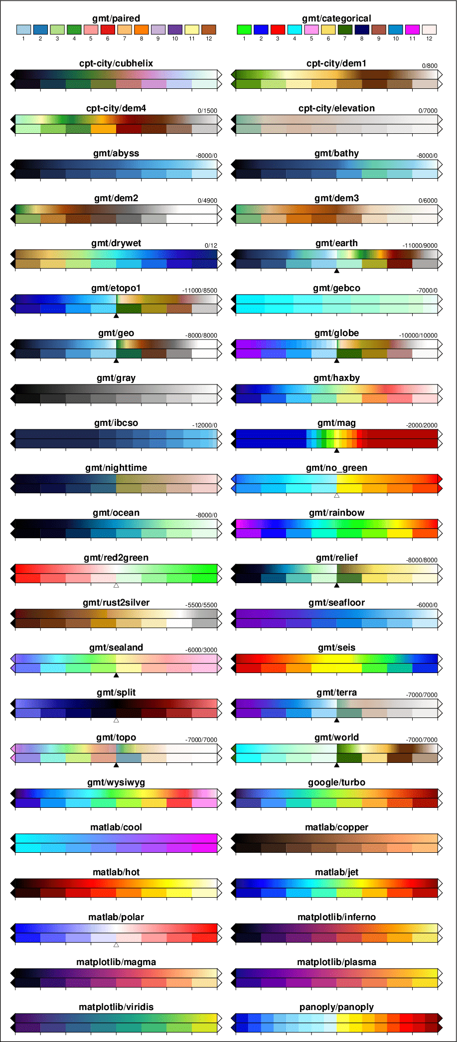
The standard CPTs supported by GMT.
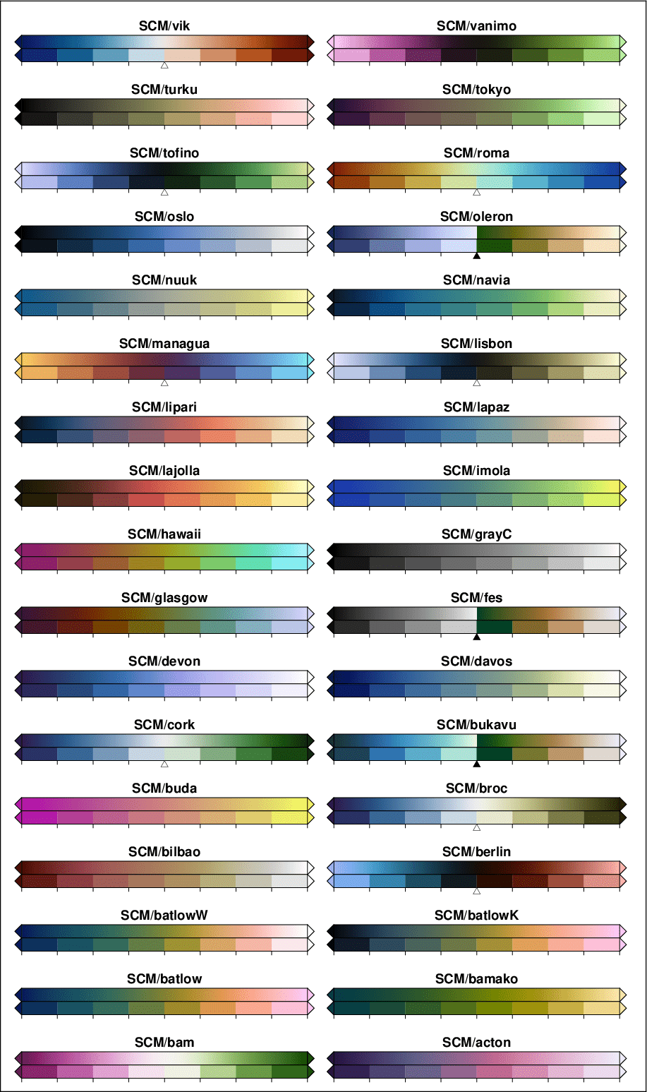
The color maps (v8.0.1) by Fabio Crameri supported by GMT. Only the non-cyclic and non-categorical variants are shown here.
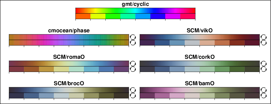
The categorical (top row) and cyclic color maps supported by GMT. Those starting with “SCM” are the cyclic scientific color maps by Fabio Crameri; those stating with “cmocean” are cyclic color maps by Kristen M. Thyng. Note: Any GMT colormap can be made cyclic by running makecpt with the -Ww option (wrapped = cyclic).
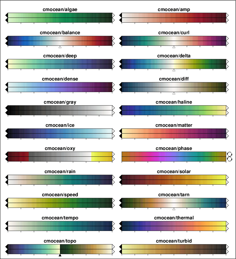
The color maps from cmocean by Kristen M. Thyng supported by GMT.
For additional color tables, visit cpt-city and Scientific Colour-Maps.
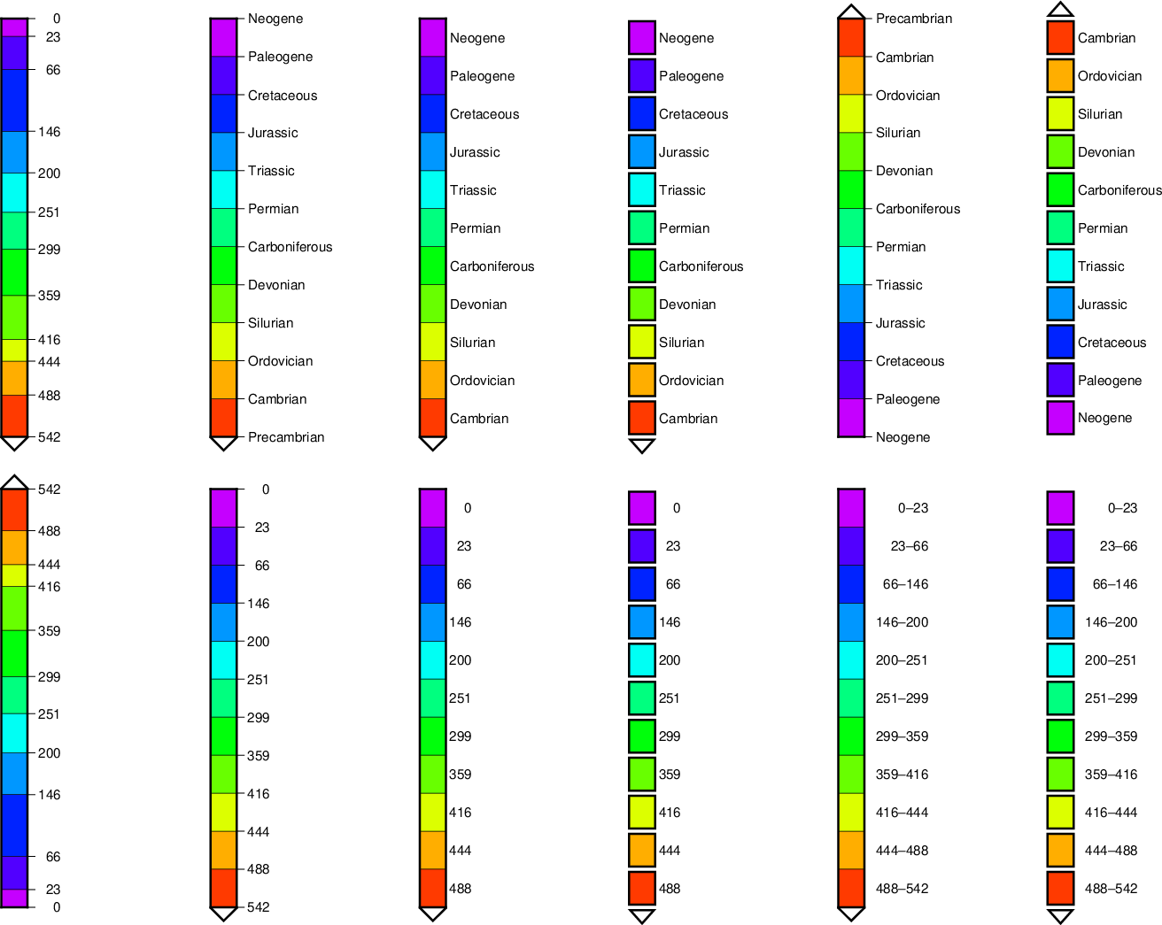
17.2. Labeled and non-equidistant color legends
The use of color legends has already been introduced in Examples 2, 16, and 17. Things become a bit more complicated when you want to label the legend with names for certain intervals (like geological time periods in the example below). To accomplish that, one should add a semi-colon and the label name at the end of a line in the CPT and add the -L option to the colorbar command that draws the color legend. This option also makes all intervals in the legend of equal length, even it the numerical values are not equally spaced.
Normally, the name labels are plotted at the lower end of the intervals. But by adding a gap amount (even when zero) to the -L option, they are centered. The example below also shows how to annotate ranges using -Li (in which case no name labels should appear in the CPT), and how to switch the color bar around (by using a negative length).
Note: If the last slice should have both lower and upper custom labels then you must supply two semicolon-separated labels and set the annotation code to B.