polar
Plot polarities on the lower hemisphere of the focal sphere
Synopsis
gmt polar [ table ] -Dlon/lat -Jparameters -Rregion -Msize[+mmag] -S<symbol><size> [ -B[p|s]parameters ] [ -Efill ] [ -Ffill ] [ -Gfill ] [ -N ] [ -Qmode[args] ] [ -T[+aangle][+ffont][+jjustify][+odx[/dy]] ] [ -U[stamp] ] [ -V[level] ] [ -Wpen ] [ -X[a|c|f|r][xshift] ] [ -Y[a|c|f|r][yshift] ] [ -dinodata[+ccol] ] [ -eregexp ] [ -hheaders ] [ -iflags ] [ -qiflags ] [ -ttransp ] [ -:[i|o] ] [ --PAR=value ]
Description
Plot observations from a single earthquake observed at various stations at different azimuths and distances on the lower hemisphere of the focal sphere. The focal sphere is typically plotted at the location of the earthquake, specified via -D. Reads data values from files [or standard input].
Parameters are expected to be in the following columns:
- 1,2,3:
station-code azimuth take-off-angle (all three columns must contain numerical values)
- 4:
polarity:
compression can be c,C,u,U,+
rarefaction can be d,D,r,R,-
not defined is anything else
Required Arguments
- table
One or more ASCII (or binary, see -bi[ncols][type]) data table file(s) holding a number of data columns. If no tables are given then we read from standard input.
- -Dlon/lat
Centers the focal sphere at given longitude and latitude point on the map.
- -Jparameters
Specify the projection. (See full description) (See cookbook summary) (See projections table).
- -Msize[+mmag]
Sets the size of the focal sphere to plot polarities in. size is in default units (unless c, i, or p is appended). Optionally append +mmag to specify its magnitude, then focal sphere size is mag / 5.0 * size.
-Rwest/east/south/north[/zmin/zmax][+r][+uunit]
Specify the region of interest. Note: If using modern mode and -R is not provided, the region will be set based on previous plotting commands. If this is the first plotting command in the modern mode levels and -R is not provided, the region will be automatically determined based on the data in table (equivalent to using -Ra). (See full description) (See cookbook information).
The region may be specified in one of several ways:
-Rwest/east/south/north. This is the standard way to specify geographic regions when using map projections where meridians and parallels are rectilinear. The coordinates may be specified in decimal degrees or in [±]dd:mm[:ss.xxx][W|E|S|N] format.
-Rwest/south/east/north+r. This form is useful for map projections that are oblique, making meridians and parallels poor choices for map boundaries. Here, we instead specify the lower left corner and upper right corner geographic coordinates, followed by the modifier +r. This form guarantees a rectangular map even though lines of equal longitude and latitude are not straight lines.
-Rg or -Rd. These forms can be used to quickly specify the global domain (0/360 for -Rg and -180/+180 for -Rd in longitude, with -90/+90 in latitude).
-Rcode1,code2,…[+e|r|Rincs]. This indirectly supplies the region by consulting the DCW (Digital Chart of the World) database and derives the bounding regions for one or more countries given by the codes. Simply append one or more comma-separated countries using either the two-character ISO 3166-1 alpha-2 convention (e.g., NO) or the full country name (e.g., Norway). To select a state within a country (if available), append .state (e.g, US.TX), or the full state name (e.g., Texas). To specify a whole continent, spell out the full continent name (e.g., -RAfrica). Finally, append any DCW collection abbreviations or full names for the extent of the collection or named region. All names are case-insensitive. The following modifiers can be appended:
+r to adjust the region boundaries to be multiples of the steps indicated by inc, xinc/yinc, or winc/einc/sinc/ninc [default is no adjustment]. For example, -RFR+r1 will select the national bounding box of France rounded to nearest integer degree, where inc can be positive to expand the region or negative to shrink the region.
+R to adjust the region by adding the amounts specified by inc, xinc/yinc, or winc/einc/sinc/ninc [default is no extension], where inc can be positive to expand the region or negative to shrink the region.
+e to adjust the region boundaries to be multiples of the steps indicated by inc, xinc/yinc, or winc/einc/sinc/ninc, while ensuring that the bounding box is adjusted by at least 0.25 times the increment [default is no adjustment], where inc can be positive to expand the region or negative to shrink the region.
-Rxmin/xmax/ymin/ymax[+uunit] specifies a region in projected units (e.g., UTM meters) where xmin/xmax/ymin/ymax are Cartesian projected coordinates compatible with the chosen projection (-J) and unit is an allowable distance unit [e]; we inversely project to determine the actual rectangular geographic region. For projected regions centered on (0,0) you may use the short-hand -Rhalfwidth[/halfheight]+uunit, where halfheight defaults to halfwidth if not given. This short-hand requires the +u modifier.
-Rjustifylon0/lat0/nx/ny, where justify is a 2-character combination of L|C|R (for left, center, or right) and T|M|B (for top, middle, or bottom) (e.g., BL for lower left). The two character code justify indicates which point on a rectangular region region the lon0/lat0 coordinates refer to and the grid dimensions nx and ny are used with grid spacings given via -I to create the corresponding region. This method can be used when creating grids. For example, -RCM25/25/50/50 specifies a 50x50 grid centered on 25,25.
-Rgridfile. This will copy the domain settings found for the grid in specified file. Note that depending on the nature of the calling module, this mechanism will also set grid spacing and possibly the grid registration (see Grid registration: The -r option).
-Ra[uto] or -Re[xact]. Under modern mode, and for plotting modules only, you can automatically determine the region from the data used. You can either get the exact area using -Re [Default if no -R is given] or a slightly larger area sensibly rounded outwards to the next multiple of increments that depend on the data range using -Ra.
- -S<symbol_type><size>
Selects symbol_type and symbol size. Size is in default units (unless c, i, or p is appended). Choose symbol type from st(a)r, (c)ircle, (d)iamond, (h)exagon, (i)nverted triangle, (p)oint, (s)quare, (t)riangle, (x)cross.
Optional Arguments
- -B[p|s]parameters
Set map boundary frame and axes attributes. (See full description) (See cookbook information).
- -Efill (more …)
Selects filling of symbols for stations in extensive quadrants. Set the color [Default is 250]. If -Efill is the same as -Ffill, use -Qe to outline.
- -Ffill (more …)
Sets background color of the focal sphere. Default is no fill.
- -Gfill (more …)
Selects filling of symbols for stations in compressional quadrants. Set the color [Default is black].
- -N
Does not skip symbols that fall outside map border [Default plots points inside border only].
- -Qmode[args]
Sets one or more attributes; repeatable. The various combinations are
- -Qe[pen]
Outline symbols in extensive quadrants using pen or the default pen (see -W).
- -Qf[pen]
Outline the focal sphere using pen or the default pen (see -W).
- -Qg[pen]
Outline symbols in compressional quadrants using pen or the default pen (see -W).
- -Qh
Use special format derived from HYPO71 output
- -Qshalf-size[+vv_size[vecspecs]]
Plots S polarity azimuth. S polarity is in last column. Append +v to select a vector and append head size and any vector specifications. If +v is given without arguments then we default to +v0.3i+e+gblack [Default is a line segment]. Give half-size in default units (unless c, i, or p is appended). See Vector Attributes for specifying additional attributes.
- -Qtpen
Set pen color to write station code. Default uses the default pen (see -W).
- -T[+aangle][+ffont][+jjustify][+odx[/dy]]
Write station code near symbols.
Optionally append +aangle to change the text angle; +ffont to set the font of the text; append +jjustify to change the text location relative to the symbol; append +o to offset the text string by dx/dy. [Default to write station code above the symbol; the default font size is 12p]
- -U[label|+c][+jjust][+odx[/dy]]
Draw GMT time stamp logo on plot. (See full description) (See cookbook information).
- -V[level]
Select verbosity level [w]. (See full description) (See cookbook information).
- -W[-|+][pen][attr] (more …)
Set current pen attributes [Default pen is default,black,solid].
- -X[a|c|f|r][xshift]
Shift plot origin. (See full description) (See cookbook information).
- -Y[a|c|f|r][yshift]
Shift plot origin. (See full description) (See cookbook information).
- -dinodata[+ccol] (more …)
Replace input columns that equal nodata with NaN.
- -e[~]“pattern” | -e[~]/regexp/[i] (more …)
Only accept data records that match the given pattern.
- -icols[+l][+ddivisor][+sscale|d|k][+ooffset][,…][,t[word]] (more …)
Select input columns and transformations (0 is first column, t is trailing text, append word to read one word only).
- -qi[~]rows|limits[+ccol][+a|t|s] (more …)
Select input rows or data limit(s) [default is all rows].
- -ttransp[/transp2] (more …)
Set transparency level(s) in percent.
- -:[i|o] (more …)
Swap 1st and 2nd column on input and/or output.
- -^ or just -
Print a short message about the syntax of the command, then exit (Note: on Windows just use -).
- -+ or just +
Print an extensive usage (help) message, including the explanation of any module-specific option (but not the GMT common options), then exit.
- -? or no arguments
Print a complete usage (help) message, including the explanation of all options, then exit.
- --PAR=value
Temporarily override a GMT default setting; repeatable. See gmt.conf for parameters.
Vector Attributes
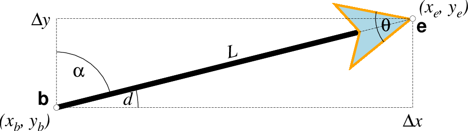
Vector attributes are controlled by options and modifiers. We will refer to this figure and the labels therein when introducing the corresponding modifiers. All vectors require you to specify the begin point \(x_b, y_b\) and the end point \(x_e, y_e\), or alternatively the direction d and length L, while for map projections we usually specify the azimuth \(\alpha\) instead.
Several modifiers may be appended to vector-producing options for specifying the placement of vector heads, their shapes, and the justification of the vector. Below, left and right refers to the side of the vector line when viewed from the beginning point (b) to the end point (e) of a line segment:
+aangle sets the angle \(\theta\) of the vector head apex [30].
+b places a vector head at the beginning of the vector path [none]. Optionally, append t for a terminal line, c for a circle, a for arrow [Default], i for tail, A for plain open arrow, and I for plain open tail. Note: For geovectors only a and A are available. Further append l|r to only draw the left or right half-sides of this head [both sides].
+c selects the vector data quantity magnitude for use with CPT color look-up [Default requires a separate data column following the 2 or 3 coordinates]. Requires that data quantity scaling (with unit q via +v or +z) and a CPT have been selected.
+e places a vector head at the end of the vector path [none]. Optionally, append t for a terminal line, c for a circle, a for arrow [Default], i for tail, A for plain open arrow, and I for plain open tail. Note: For geovectors only a and A are available. Further append l|r to only draw the left or right half-sides of this head [both sides].
+g[fill] sets the vector head fill [Default fill is used, which may be no fill]. Turn off vector head fill by not appending a fill. Some modules have a separate -Gfill option and if used will select the fill as well.
+hshape sets the shape of the vector head (range -2/2). Default is controlled by MAP_VECTOR_SHAPE [default is theme dependent]. A zero value produces no notch. Positive values moves the notch toward the head apex while a negative value moves it away. The example above uses +h0.5.
+m places a vector head at the mid-point the vector path [none]. Append f or r for forward or reverse direction of the vector [forward]. Optionally, append t for a terminal line, c for a circle, a for arrow [Default], i for tail, A for plain open arrow, and I for plain open tail. Further append l|r to only draw the left or right half-sides of this head [both sides]. Cannot be combined with +b or +e.
+n[norm[/min]] scales down vector attributes (pen thickness, head size) with decreasing length, where vector plot lengths shorter than norm will have their attributes scaled by length/norm [other arrow attributes remain invariant to length]. Optionally, append /min for the minimum shrink factor (in the 0-1 range) that we will shrink to [0.25]. For Cartesian vectors, please specify a norm in plot units, while for geovectors specify a norm in map units (see Distance units) [k]. Alternatively, append unit q to indicate we should use user quantity units in making the decision; this means the user also must select user quantity input via +v or +z.
If no argument is given then +n ensures vector heads are not shrunk and always plotted regardless of vector length [Vector heads are not plotted if exceeding vector length].
+o[plon/plat] specifies the oblique pole for the great or small circles. Only needed for great circles if +q is given. If no pole is appended then we default to the north pole. Input arguments are then lon lat arclength with the latter in map distance units; see +q of angular limits instead.
+p[pen] sets the vector pen attributes. If no pen is appended then the head outline is not drawn. [Default pen is half the width of stem pen, and head outline is drawn]. Above, we used +p2p,orange. The vector stem attributes are controlled by -W.
+q means the input direction, length data instead represent the start and stop opening angles of the arc segment relative to the given point. See +o to specify a specific pole for the arc [north pole].
+t[b|e]trim will shift the beginning or end point (or both) along the vector segment by the given trim; append suitable unit (c, i, or p). If the modifiers b|e are not used then trim may be two values separated by a slash, which is used to specify different trims for the beginning and end. Positive trims will shorted the vector while negative trims will lengthen it [no trim].
In addition, all but circular vectors may take these modifiers:
+jjust determines how the input x,y point relates to the vector. Choose from beginning [default], end, or center.
+s means the input angle, length are instead the \(x_e, y_e\) coordinates of the vector end point.
Finally, Cartesian vectors and geovectors may take these modifiers (except in grdvector) which can be used to convert vector components to polar form or magnify user quantity magnitudes into plot lengths.
+v[i|l]scale expects a scale to magnify the polar length in the given unit. If i is prepended we use the inverse scale while if l is prepended then it is taken as a fixed length to override input lengths. Append unit q if input magnitudes are given in user quantity units and we will scale them to current plot unit for Cartesian vectors (see PROJ_LENGTH_UNIT for how to change the plot unit) or to km for geovectors. In addition, if +c is selected then the vector magnitudes may be used for CPT color-lookup (and no extra data column is required by -C).
+z[scale] expects input \(\Delta x, \Delta y\) vector components and uses the scale [1] to convert to polar coordinates with length in given unit. Append unit q if input components are given in user quantity units and we will scale to current plot unit for Cartesian vectors (see PROJ_LENGTH_UNIT for how to change the plot unit) or to km for geovectors. In addition, if +c is selected then the vector magnitudes may be used for CPT color-lookup (and no extra data column is required by -C).
Note: Vectors were completely redesigned for GMT5 which separated the vector head (a polygon) from the vector stem (a line). In GMT4, the entire vector was a polygon and it could only be a straight Cartesian vector. Yes, the old GMT4 vector shape remains accessible if you specify a vector (-Sv|V) using the GMT4 syntax, explained here: size, if present, will be interpreted as \(t_w/h_l/h_w\) or tailwidth/headlength/halfheadwidth [Default is 0.075c/0.3c/0.25c (or 0.03i/0.12i/0.1i)]. By default, arrow attributes remain invariant to the length of the arrow. To have the size of the vector scale down with decreasing size, append +nnorm, where vectors shorter than norm will have their attributes scaled by length/norm. To center the vector on the balance point, use -Svb; to align point with the vector head, use -Svh; to align point with the vector tail, use -Svt [Default]. To give the head point’s coordinates instead of direction and length, use -Svs. Upper case B, H, T, S will draw a double-headed vector [Default is single head]. Note: If \(h_l/h_w\) are given as 0/0 then only the head-less vector stick will be plotted.
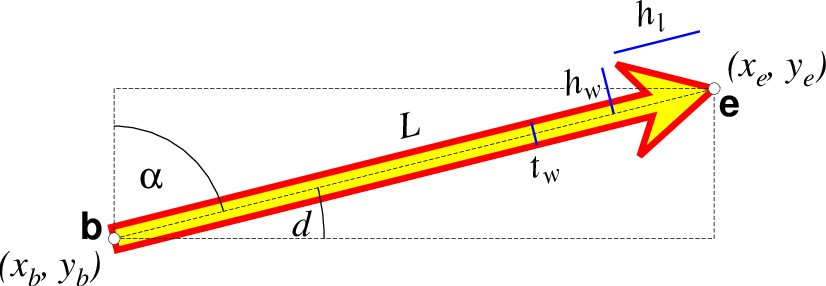
A GMT 4 vector has no separate pen for the stem -- it is all part of a Cartesian polygon. You may optionally fill and draw its outline. The modifiers listed above generally do not apply. Note: While the tailwidth (\(t_w\)) and headlength (\(h_l\)) parameters are given as indicated, the halfheadwidth (\(h_w\)) is oddly given as the half-width in GMT 4 so we retain that convention here (but have updated the documentation; blue lines indicate these three parameters).
Examples
Note: Since many GMT plot examples are very short (i.e., one module call between the gmt begin and gmt end commands), we will often present them using the quick modern mode GMT Modern Mode One-line Commands syntax, which simplifies such short scripts.
gmt polar -R239/240/34/35.2 -JM8c -N -Sc0.4 -D239.5/34.5 -M5 -pdf test << END
#stat azim ih pol
0481 11 147 c
6185 247 120 d
0485 288 114 +
0490 223 112 -
0487 212 109 .
END
Use special format derived from HYPO71 output:
gmt polar -R239/240/34/35.2 -JM8c -N -Sc0.4 -D239:30E/34:30N -M5 -Qh -pdf test <<END
#Date Or. time stat azim ih
910223 1 22 0481 11 147 ipu0
910223 1 22 6185 247 120 ipd0
910223 1 22 0485 288 114 epu0
910223 1 22 0490 223 112 epd0
910223 1 22 0487 212 109 epu0
END
References
Aki, K., & Richards, P. G. (1980). Quantitative seismology: theory and methods. San Francisco: W. H. Freeman.
Dahlen, F. A., & Tromp, J. (1998). Theoretical global seismology. Princeton, N.J: Princeton University Press.
Frohlich, C. (1996). Cliff’s Nodes Concerning Plotting Nodal Lines for P, SH and SV. Seismological Research Letters, 67(1), 16–24. https://doi.org/10.1785/gssrl.67.1.16
Lay, T., & Wallace, T. C. (1995). Modern global seismology. San Diego: Academic Press.