5. GMT Coordinate Transformations¶

GMT programs read real-world coordinates and convert them to positions on a plot. This is achieved by selecting one of several coordinate transformations or projections. We distinguish between three sets of such conversions:

Cartesian coordinate transformations
Polar coordinate transformations
Map coordinate transformations

The next Chapter will be dedicated to GMT map projections in its entirety. Meanwhile, the present Chapter will summarize the properties of the Cartesian and Polar coordinate transformations available in GMT, list which parameters define them, and demonstrate how they are used to create simple plot axes. We will mostly be using basemap (and occasionally plot) to demonstrate the various transformations. Our illustrations may differ from those you reproduce with the same commands because of different settings in our gmt.conf file.) Finally, note that while we will specify dimensions in inches (by appending i), you may want to use cm (c), or points (p) as unit instead (see the gmt.conf man page).

5.1. Cartesian transformations¶

GMT Cartesian coordinate transformations come in three flavors:

Linear coordinate transformation
Log\(_{10}\) coordinate transformation
Power (exponential) coordinate transformation

These transformations convert input coordinates (x,y) to locations (x’, y’) on a plot. There is no coupling between x and y (i.e., x’ = f(x) and y’ = f(y)); it is a one-dimensional projection. Hence, we may use separate transformations for the x- and y-axes (and z-axes for 3-D plots). Below, we will use the expression u’ = f(u), where u is either x or y (or z for 3-D plots). The coefficients in f(u) depend on the desired plot size (or scale), the chosen (x,y) domain, and the nature of f itself.

Two subsets of linear will be discussed separately; these are a polar (cylindrical) projection and a linear projection applied to geographic coordinates (with a 360° periodicity in the x-coordinate). We will show examples of all of these projections using dummy data sets created with gmtmath, a “Reverse Polish Notation” (RPN) calculator that operates on or creates table data:

gmt math -T0/100/1  T SQRT = sqrt.txt
gmt math -T0/100/10 T SQRT = sqrt10.txt

5.1.1. Cartesian linear transformation (-Jx -JX)¶

There are in fact three different uses of the Cartesian linear transformation, each associated with specific command line options. The different manifestations result from specific properties of three kinds of data:

Regular floating point coordinates
Geographic coordinates
Calendar time coordinates

Examples of Cartesian (left), circular (middle), and geo-vectors (right) for different attribute specifications. Note that both full and half arrow-heads can be specified, as well as no head at all.

5.1.1.1. Regular floating point coordinates¶

Selection of the Cartesian linear transformation with regular floating point coordinates will result in a simple linear scaling u’ = au + b of the input coordinates. The projection is defined by stating scale in inches/unit (-Jx) or axis length in inches (-JX). If the y-scale or y-axis length is different from that of the x-axis (which is most often the case), separate the two scales (or lengths) by a slash, e.g., -Jx0.1i/0.5i or -JX8i/5i. Thus, our \(y = \sqrt{x}\) data sets will plot as shown in Figure Linear transformation of Cartesian coordinates.

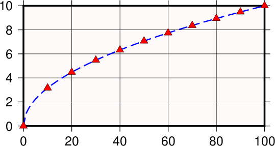
Linear transformation of Cartesian coordinates.¶

The complete commands given to produce this plot were

gmt begin GMT_linear
	gmt plot -R0/100/0/10 -JX8c/4c -Bag -BWSne+gsnow -Wthick,blue,- sqrt.txt
	gmt plot -St0.3c -N -Gred -Wfaint sqrt10.txt
gmt end show

Normally, the user’s x-values will increase to the right and the y-values will increase upwards. It should be noted that in many situations it is desirable to have the direction of positive coordinates be reversed. For example, when plotting depth on the y-axis it makes more sense to have the positive direction downwards. All that is required to reverse the sense of positive direction is to supply a negative scale (or axis length). Finally, sometimes it is convenient to specify the width (or height) of a map and let the other dimension be computed based on the implied scale and the range of the other axis. To do this, simply specify the length to be recomputed as 0.

5.1.1.2. Geographic coordinates¶

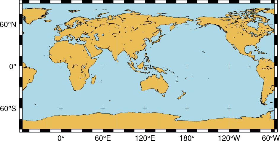
Linear transformation of map coordinates.¶

While the Cartesian linear projection is primarily designed for regular floating point x,y data, it is sometimes necessary to plot geographical data in a linear projection. This poses a problem since longitudes have a 360° periodicity. GMT therefore needs to be informed that it has been given geographical coordinates even though a linear transformation has been chosen. We do so by adding a g (for geographical) or d (for degrees) directly after -R or by appending a g or d to the end of the -Jx (or -JX) option. As an example, we want to plot a crude world map centered on 125°E. Our command will be

gmt begin GMT_linear_d
	gmt set MAP_GRID_CROSS_SIZE_PRIMARY 0.1i MAP_FRAME_TYPE FANCY FORMAT_GEO_MAP ddd:mm:ssF
	gmt coast -Rg-55/305/-90/90 -Jx0.04c -Bagf -BWSen -Dc -A1000 -Glightbrown -Wthinnest -Slightblue
gmt end show

with the result reproduced in Figure Linear transformation of map coordinates.

5.1.1.3. Calendar time coordinates¶

Linear transformation of calendar coordinates.¶

Several particular issues arise when we seek to make linear plots using calendar date/time as the input coordinates. As far as setting up the coordinate transformation we must indicate whether our input data have absolute time coordinates or relative time coordinates. For the former we append T after the axis scale (or width), while for the latter we append t at the end of the -Jx (or -JX) option. However, other command line arguments (like the -R option) may already specify whether the time coordinate is absolute or relative. An absolute time entry must be given as [date]T[clock] (with date given as yyyy[-mm[-dd]], yyyy[-jjj], or yyyy[-Www[-d]], and clock using the hh[:mm[:ss[.xxx]]] 24-hour clock format) whereas the relative time is simply given as the units of time since the epoch followed by t (see TIME_UNIT and TIME_EPOCH for information on specifying the time unit and the epoch). As a simple example, we will make a plot of a school week calendar (Figure Linear transformation of calendar coordinates).

When the coordinate ranges provided by the -R option and the projection type given by -JX (including the optional d, g, t or T) conflict, GMT will warn the users about it. In general, the options provided with -JX will prevail.

gmt begin GMT_linear_cal
	gmt set FORMAT_DATE_MAP o TIME_WEEK_START Sunday FORMAT_CLOCK_MAP=-hham FORMAT_TIME_PRIMARY_MAP full
	gmt basemap -R2001-9-24T/2001-9-29T/T07:0/T15:0 -JX10c/-5c -Bxa1Kf1kg1d -Bya1Hg1h -BWsNe+glightyellow
gmt end show

5.1.2. Cartesian logarithmic projection¶

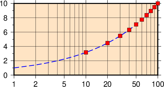
Logarithmic transformation of x–coordinates.¶

The \(\log_{10}\) transformation is simply \(u' = a \log_{10}(u) + b\) and is selected by appending an l (lower case L) immediately following the scale (or axis length) value. Hence, to produce a plot in which the x-axis is logarithmic (the y-axis remains linear, i.e., a semi-log plot), try (Figure Logarithmic transformation)

gmt begin GMT_log
	gmt plot -R1/100/0/10 -Jx4cl/0.4c -Bx2g3 -Bya2f1g2 -BWSne+gbisque -Wthick,blue,- -h sqrt.txt
	gmt plot -Ss0.3c -N -Gred -W -h sqrt10.txt
gmt end show

Note that if x- and y-scaling are different and a \(\log_{10}-\log_{10}\) plot is desired, the l must be appended twice: Once after the x-scale (before the /) and once after the y-scale.

5.1.3. Cartesian power projection …¶

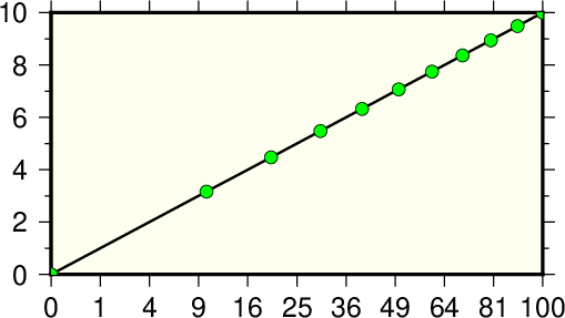
Exponential or power transformation of x–coordinates.¶

This projection uses \(u' = a u^b + c\) and allows us to explore exponential relationships like \(x^p\) versus \(y^q\). While p and q can be any values, we will select p = 0.5 and q = 1 which means we will plot x versus \(\sqrt{x}\). We indicate this scaling by appending a p (lower case P) followed by the desired exponent, in our case 0.5. Since q = 1 we do not need to specify p1 since it is identical to the linear transformation. Thus our command becomes (Figure Power transformation)

gmt begin GMT_pow
	gmt plot -R0/100/0/10 -Jx0.75cp0.5/0.4c -Bxa1p -Bya2f1 -BWSne+givory -Wthick sqrt.txt
	gmt plot -Sc0.2c -Ggreen -W sqrt10.txt
gmt end show

5.2. Linear projection with polar coordinates (-Jp -JP) …¶

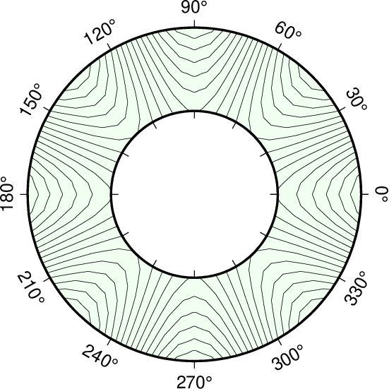
Polar (Cylindrical) transformation of (\(\theta, r\)) coordinates.¶

This transformation converts polar coordinates (angle \(\theta\) and radius r) to positions on a plot. Now \(x' = f(\theta,r)\) and \(y' = g(\theta,r)\), hence it is similar to a regular map projection because x and y are coupled and x (i.e., \(\theta\)) has a 360° periodicity. With input and output points both in the plane it is a two-dimensional projection. The transformation comes in several flavors:

Normally, \(\theta\) is understood to be directions counter-clockwise from the horizontal axis, but we may choose to specify an angular offset [whose default value is zero]. We will call this offset \(\theta_0\). Then, \(x' = f(\theta, r) = ar \cos (\theta-\theta_0) + b\) and \(y' = g(\theta, r) = ar \sin (\theta-\theta_0) + c\).
Alternatively, \(\theta\) can be interpreted to be azimuths clockwise from the vertical axis, yet we may again choose to specify the angular offset [whose default value is zero]. Then, \(x' = f(\theta, r) = ar \cos (90 - (\theta-\theta_0)) + b\) and \(y' = g(\theta, r) = ar \sin (90 - (\theta-\theta_0)) + c\).
The radius r can either be radius or inverted to mean depth from the surface, planetary radii, or even elevations in degrees.

Consequently, the polar transformation is defined by providing

scale in inches/unit (-Jp) or full width of plot in inches (-JP)
Optionally, append +a to indicate CW azimuths rather than CCW directions
Optionally, append +torigin in degrees so that this angular value is aligned with the positive x-axis (or the azimuth to be aligned with the positive y-axis if +a) [0].
Optionally, append +f to flip the radial direction to point inwards, and append e to indicate that r represents elevations in degrees (requires south >= 0 and north <= 90), p to select current planetary radius (determined by PROJ_ELLIPSOID) as maximum radius [north], or radius to specify a custom radius.
Optionally, append +roffset to include a radial offset in measurement units [0].
Optionally, append +z to annotate depths rather than radius. Alternatively, if your r data are actually depths then you can append p or radius to get radial annotations (r = radius - z) instead.

As an example of this projection we will create a gridded data set in polar coordinates \(z(\theta, r) = r^2 \cdot \cos{4\theta}\) using grdmath, a RPN calculator that operates on or creates grid files.

gmt begin GMT_polar
	gmt grdmath -R0/360/2/4 -I6/0.1 X 4 MUL PI MUL 180 DIV COS Y 2 POW MUL = tt.nc
	gmt grdcontour tt.nc -JP8c -B30 -BNs+ghoneydew -C2 -S4 --FORMAT_GEO_MAP=+ddd
gmt end show

We used grdcontour to make a contour map of this data. Because the data file only contains values with \(2 \leq r \leq 4\), a donut shaped plot appears in Figure Polar transformation.