(51) OpenStreetMap coastlines in GMT

This example shows how to use coastlines derived from the OpenStreetMap (OSM) project in GMT. When working with the high resolution SRTM Datasets provided by GMT, the GSHHG coastlines might not be precise enough on small scales. Here comes the OSM project to the rescue as it provides high resolution coastlines in the WGS84 datum. Not as convenient and fast as GSHHG but easy enough to give it a try – as long as you have space on your hard drive and some processor cycles to spare.

Note

This example makes use of data provided by third parties outside the GMT universe. As the internet is constantly changing, the source of this data might move or vanish altogether.

First we need to download the appropriate shape file. The OSM Wiki has some sources, this is the one we are going to use. The nice people of the German FOSSGIS society already did some of the heavylifting and converted the OSM coastlines to a shape file for us. Make sure to get the Land Polygon in the Large polygons not split version with WGS84 datum from their download page. It’s a ~630 MB download.

You may use this file right away as GMT converts it under the hood to something more useful on the fly. Neither very fast nor very efficient if you want to use the file multiple times and have to deal with large file sizes as we do here. So we use GDAL’s ogr2ogr and convert the shape file to a native GMT format.

As the resulting raw ASCII file is very large (>1 GB), GMT’s convert is used to reduce the file size to a third by converting it to a single-precision binary file. The resulting file is smaller than the initial download while still maintaining precision in the range of centimeters.

To speed up the plotting process even more, we extract the region of interest with select. Finally we are all set to use the coastlines with plot to get nice, precise coastlines in our illustrations.

#!/usr/bin/env bash
# GMT EXAMPLE 51
#
# Purpose:     Illustrate usage of OpenStreetMap coastlines in GMT
# GMT modules: convert, select, coast, plot
# GDAL progs:  ogr2ogr


# First we convert the shapefile to something more GMT friendly. Here we make it
# into a large ASCII file. Human-readable but not very efficient. GDAL's ogr2ogr
# is used with the "-f OGR_GMT" option indicating that the output should have
# the native GMT format. Input is the downloaded land_polygons.shp, and the
# output is named land_polygons_osm_planet.gmt. The resulting file is very
# large (>1 GB) but already usable. But wait, there is more ...

ogr2ogr -f OGR_GMT land_polygons_osm_planet.gmt land_polygons.shp

# Resorting to GMT's convert program we take our very large ASCII file and
# reduce it to about a third of its original size by converting it to a binary
# file. Lets have a closer look at -bo2f: 
# -bo selects native binary output
# 2 makes it two data columns
# f indicates 4-byte single-precision for the data

gmt convert land_polygons_osm_planet.gmt -bo2f > land_polygons_osm_planet.bf2

# Now the heavylifting is done and we have a reusable global coastline file
# with higher precision than the GSHHG coastlines.
# Again, we could use the file as is, but there are more performance gains to
# collect. We extract just the area we need for our plot. Here the island of
# Sao Vicente, Cape Verde. select to the rescue! -bo2f is nothing new and -bi2f
# looks very similar: the -bi is indicating native binary input. -R...+r gives
# the area which we are interested in.

gmt select land_polygons_osm_planet.bf2 -bi2f -bo2f -R-25.14/16.75/-24.8/16.95+r > land_polygons_osm_caboverde.bf2

# Finally it is time to do the thing we are here for: Plot some OSM coastlines
# and compare them to the GSHHG coastlines.

gmt begin ex51
  
  # To make the lines a bit nicer we set the line endcaps and the way lines are
  # joined to round
  
  gmt set PS_LINE_CAP round
  gmt set PS_LINE_JOIN round
  
  # To get an idea where the GSHHG coastlines are we lay them down first with a
  # thin red pen. -JL defines a Lambert conic conformal projection and -R...+r
  # is the area of the plot. -W defines the pen and -B the style of the plot
  # borders, gridlines and annotations. 
  
  gmt coast -JL-24.9/16.55/16.3/16.7/15c -R-25.14/16.75/-24.8/16.95+r -Wred -Ba10mg10m
  
  # Time to use the OSM coastlines we prepared earlier. Straightforward we
  # supply the extracted area, tell plot about the binary format (-bi), define
  # pen (-W) and fill (-G)
  
  gmt plot land_polygons_osm_caboverde.bf2 -bi2f -Wthinnest,black -Ggrey
  
  # Here we plot the GSHHG coastlines a second time but now with a dashed pen
  # to highlight the areas where they would otherwise be hidden behind the grey
  # OSM landmass. 
  
  gmt coast -Wred,dashed
  
gmt end show

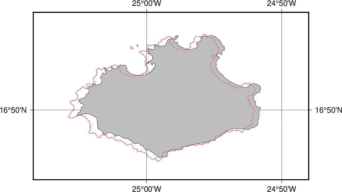
../_images/ex51.png — Comparison of GSHHG and OSM coastlines.