grdflexure
Compute flexural deformation of 3-D surfaces for various rheologies
Synopsis
gmt grdflexure topogrd -Drm/rl[/ri]/rw -E[Te[k][/Te2[k]]] -Goutgrid [ -ANx/Ny/Nxy ] [ -Cp|yvalue ] [ -Fnu_a[/h_a[k]/nu_m] ] [ -Llist ] [ -Mtm ] [ -Nparams ] [ -Q ] [ -Sbeta ] [ -Tt0[/t1/dt[+l]]|file ] [ -V[level] ] [ -Wwd][k] [ -Zzm][k] [ -fflags ] [ --PAR=value ]
Note: No space is allowed between the option flag and the associated arguments.
Description
grdflexure computes the deformation due to a topographic load \(h(\mathbf{x})\) for five different types of rheological foundations, all involving constant thickness thin plates:
An elastic plate overlying an inviscid half-space,
An elastic plate overlying a viscous half-space (Firmoviscous or Kelvin-Voigt),
An elastic plate overlying a viscous layer over a viscous half-space (Firmoviscous or Kelvin-Voigt),
A viscoelastic plate overlying an inviscid half-space (Maxwell solid),
A general linear viscoelastic model with an initial and final elastic plate thickness overlying an inviscid half-space.
These conditions will require the elastic [1; \(\Phi_e(\mathbf{k})\)], firmoviscous [2,3; \(\Phi_{fv}(\mathbf{k},t)\)], viscoelastic [4; \(\Phi_{ve}(\mathbf{k},t)\)], and general linear (viscoelastic) response functions [5; \(\Phi_{gl}(\mathbf{k},t)\)] If the (visco)elastic plate vanishes (zero thickness) then we obtain Airy isostasy (1,4) or a purely viscous response (2,3). Temporal evolution can also be modeled by providing incremental load grids for select times and specifying a range of model output times. A wide range of options allow specifying the desired rheology and related constants, including in-plate forces.
Required Arguments
- topogrd
2-D binary grid file with the topography of the load (in meters); (See Grid File Formats). If -T is used, topogrd may be a filename template with a floating point format (C syntax) and a different load file name will be set and loaded for each time step. The load times thus coincide with the times given via -T (but not all times need to have a corresponding file). Alternatively, give topogrd as =flist, where flist is an ASCII table with one topogrd filename and load time per record. These load times can be different from the evaluation times given via -T. For load time format, see -T. Note: If flist has an optional third column it will be interpreted as a load density and used for that layer instead of the fixed rl setting in -D.
- -Drm/rl[/ri]/rw
Sets density for mantle, load, infill, and water (or air). If ri differs from rl then an approximate solution will be found. If ri is not given then it defaults to rl. Values may be given in km/m^3 or g/cm^3.
- -E[Te[k][/Te2[k]]
Sets the elastic plate thickness (in meter); append k for km. If the elastic thickness exceeds 1e10 it will be interpreted as a flexural rigidity D (by default, D is computed from Te, Young’s modulus, and Poisson’s ratio; see -C to change these values). If just -E is given and -F is used it means no plate is given and we will return a purely viscous response with or without an asthenospheric layer. Select a general linear viscoelastic response by supplying both an initial and final elastic thickness; this response also requires -M.
-Goutgrid[=ID][+ddivisor][+ninvalid] [+ooffset|a][+sscale|a] [:driver[dataType][+coptions]]
If -T is set then outgrid must be a filename template that contains a floating point format (C syntax). If the filename template also contains either %s (for unit name) or %c (for unit letter) then we use the corresponding time (in units specified in -T) to generate the individual file names, otherwise we use time in years with no unit. Optionally, append =ID for writing a specific file format (See full description). The following modifiers are supported:
+d - Divide data values by given divisor [Default is 1].
+n - Replace data values matching invalid with a NaN.
+o - Offset data values by the given offset, or append a for automatic range offset to preserve precision for integer grids [Default is 0].
+s - Scale data values by the given scale, or append a for automatic scaling to preserve precision for integer grids [Default is 1].
Note: Any offset is added before any scaling. +sa also sets +oa (unless overridden). To write specific formats via GDAL, use = gd and supply driver (and optionally dataType) and/or one or more concatenated GDAL -co options using +c. See the “Writing grids and images” cookbook section for more details.
Optional Arguments
- -ANx/Ny/Nxy
Specify in-plane compressional or extensional forces in the x- and y-directions, as well as any shear force [no in-plane forces]. Compression is indicated by negative values, while extensional forces are specified using positive values. Values are expected in Pa·m since N is the depth-integrated horizontal stresses.
- -Cp|yvalue
Append p or y to change the current value of Poisson’s ratio [0.25] or Young’s modulus [7.0e10 N/m^2], respectively.
- -Fnu_a[/h_a[k]/nu_m]
Specify a firmoviscous model in conjunction with an elastic plate thickness specified via -E. Just give one viscosity (nu_a) for an elastic plate over a viscous half-space, or also append the thickness of the asthenosphere (h_a) and the lower mantle viscosity (nu_m), with the first viscosity now being that of the asthenosphere. Give viscosities in Pa·s. If used, give the thickness of the asthenosphere in meter; append k for km. Cannot be used in conjunctions with -M.
- -Llist
Write the names and evaluation times of all grids that were created to the text file list. Requires -T.
- -N[a|f|m|r|s|nx/ny][+a|d|h|l][+e|n|m][+twidth][+v][+w[suffix]][+z[p]]
Choose or inquire about suitable grid dimensions for FFT and set optional parameters. Control the FFT dimension:
-Na lets the FFT select dimensions yielding the most accurate result.
-Nf will force the FFT to use the actual dimensions of the data.
-Nm lets the FFT select dimensions using the least work memory.
-Nr lets the FFT select dimensions yielding the most rapid calculation.
-Ns will present a list of optional dimensions, then exit.
-Nnx/ny will do FFT on array size nx/ny (must be >= grid file size). Default chooses dimensions >= data which optimize speed and accuracy of FFT. If FFT dimensions > grid file dimensions, data are extended and tapered to zero.
Control detrending of data: Append modifiers for removing a linear trend:
+d: Detrend data, i.e. remove best-fitting linear trend [Default].
+a: Only remove mean value.
+h: Only remove mid value, i.e. 0.5 * (max + min).
+l: Leave data alone.
Control extension and tapering of data: Use modifiers to control how the extension and tapering are to be performed:
+e extends the grid by imposing edge-point symmetry [Default],
+m extends the grid by imposing edge mirror symmetry
+n turns off data extension.
Tapering is performed from the data edge to the FFT grid edge [100%]. Change this percentage via +twidth. When +n is in effect, the tapering is applied instead to the data margins as no extension is available [0%].
Control messages being reported: +v will report suitable dimensions during processing.
Control writing of temporary results: For detailed investigation you can write the intermediate grid being passed to the forward FFT; this is likely to have been detrended, extended by point-symmetry along all edges, and tapered. Append +w[suffix] from which output file name(s) will be created (i.e., ingrid_prefix.ext) [tapered], where ext is your file extension. Finally, you may save the complex grid produced by the forward FFT by appending +z. By default we write the real and imaginary components to ingrid_real.ext and ingrid_imag.ext. Append p to save instead the polar form of magnitude and phase to files ingrid_mag.ext and ingrid_phase.ext.
- -Mtm
Specify a viscoelastic model in conjunction with a plate thickness specified via -E. Append the Maxwell time tm for the viscoelastic model (in years); add k for kyr and M for Myr. Cannot be used in conjunctions with -F.
- -Q
Do not make any flexure calculations but instead take the chosen response function given the parameters you selected and evaluate it for a range of wavenumbers and times; see the note on transfer functions below.
- -Sbeta
Specify a starved moat fraction in the 0-1 range, where 1 means the moat is fully filled with material of density ri while 0 means it is only filled with material of density rw (i.e., just water) [1].
- -Tt0[/t1/dt[+l]]|file
Specify t0, t1, and time increment (dt) for a sequence of calculations [Default is one calculation, with no time dependency]. For a single specific time, just give start time t0. Default unit is years; append k for kyr and M for Myr. For a logarithmic time scale, append +l and specify n steps instead of dt. Alternatively, give a file with the desired times in the first column (these times may have individual units appended, otherwise we assume year). We then write a separate model grid file for each given time step; see -G* for output file template format.
- -V[level]
Select verbosity level [w]. (See full description) (See cookbook information).
- -Wwd[k]
Set reference water depth for the undeformed flexed surface in m. Must be positive. [0]. Append k to indicate km. If -W is used and your load exceeds this depth then we scale the subaerial part of the load to account for the change in surrounding density (air vs water).
- -Zzm[k]
Specify reference depth to flexed surface (e.g., Moho) in m; append k for km. Must be positive. [0]. We subtract this value from the flexed surface before writing the results.
- -fflags
Geographic grids (dimensions of longitude, latitude) will be converted to meters via a “Flat Earth” approximation using the current ellipsoid parameters.
- -^ or just -
Print a short message about the syntax of the command, then exit (NOTE: on Windows just use -).
- -+ or just +
Print an extensive usage (help) message, including the explanation of any module-specific option (but not the GMT common options), then exit.
- -? or no arguments
Print a complete usage (help) message, including the explanation of all options, then exit.
- --PAR=value
Temporarily override a GMT default setting; repeatable. See gmt.conf for parameters.
Grid Distance Units
If a Cartesian grid does not have meter as the horizontal unit, append +uunit to the input file name to convert from the specified unit to meter. E.g., appending +uk to the load file name will scale the grid x,y coordinates from km to meter. If your grid is geographic, convert distances to meters by supplying -fflags instead. netCDF COARDS geographic grids will automatically be recognized as geographic.
Considerations
The calculations are done using a rectangular Cartesian FFT operation. If your geographic region is close to either pole, you should consider using a Cartesian setup instead; you can always project it back to geographic using grdproject.
Transfer Functions
If -Q is given we perform no actual flexure calculations and no input data file is required. Instead, we write the chosen transfer functions \(\Phi(\mathbf{k},t)\) to 7 separate files for 7 different Te values (1, 2, 5, 10, 20, 50, and 100 km). The first two columns are always wavelength in km and wavenumber (in 1/m) for a 1:1:3000 km range. The transfer functions are evaluated for 12 different response times: 1k, 2k, 5k, 10k, 20k, 50k, 100k, 200k, 500k, 1M, 2M, and 5M years. For a purely elastic response function we only write the transfer function once per elastic thickness (in column 3). The 7 files are named grdflexure_transfer_function_te_te_km.txt, where te is replaced by the 7 elastic thicknesses in km (and 0 if -E[0] was used for a viscous response only).
Examples
We will use a Gaussian seamount load to demonstrate grdflexure. First, we make a grid of for that shape by placing a Gaussian truncated seamount at position (300,300) with a radius of 50 km and height of 5000 m:
echo 300 300 0 40 40 5000 | gmt grdseamount -R0/600/0/600+uk -I1000 -Gsmt.nc t.txt -Dk -E -F0.1 -Cg
To compute elastic plate flexure from the load smt.nc, for a 10 km thick plate with typical densities, try:
gmt grdflexure smt.nc -Gflex.nc -E10k -D2700/3300/1035
To see how in-plane stresses affect the result, we use -A. Remember that we need to depth- integrated forces, not pressures, hence we try:
gmt grdflexure smt.nc -Gflex.nc -E10k -D2700/3300/1035 -A-4e11/2e11/-1e12
To compute viscoelastic plate flexure from the load smt.nc, for a 20 km thick plate with typical densities and a Maxwell time of 40kyr, try:
gmt grdflexure smt.nc -Gflex.nc -E20k -D2700/3300/1035 -M40k
To compute firmoviscous plate flexure from the load smt.nc, for a 15 km thick plate with typical densities overlying a viscous mantle with viscosity 2e21, try:
gmt grdflexure smt.nc -Gflex.nc -E15k -D2700/3300/1035 -F2e21
To compute the general linear viscoelastic plate flexure from the load smt.nc, for an initial Te of 40 km and a final Te of 15 km with typical densities and a Maxwell time of 100 kyr, try:
gmt grdflexure smt.nc -Gflex.nc -E40k/15k -D2700/3300/1035 -M100k
To just compute the firmoviscous response functions using the specified rheological values, try:
gmt grdflexure -D3300/2800/2800/1000 -Q -F2e20
The following are not user-reproducible but shows the kind of calculations that can be done. To compute the firmoviscous response to a series of incremental loads given by file name and load time in the table l.lis at the single time 1 Ma using the specified rheological values, try:
gmt grdflexure -T1M =l.lis -D3300/2800/2800/1000 -E5k -Gflx/smt_fv_%03.1f_%s.nc -F2e20 -Nf+a
Theory of Response Functions
Deformation \(w(\mathbf{x})\) caused by topography \(h(\mathbf{x})\) applied instantaneously to the rheological foundation at time t = 0 and evaluated at a later time t is given in the Fourier domain by
where \(\mathbf{k} = (k_x, k_y)\) is the wavenumber vector, \(k_r\) its magnitude, \(H(\mathbf{k})\) is the topographic load in the wavenumber domain, A is the Airy density ratio, \(\gamma\) is a constant that depends on the infill density, and \(\Phi(\mathbf{k},t)\) is the response function for the selected rheology. The grdflexure module read one or more loads h, transforms them to H, evaluates and applies the response function, and inversely transform the results back to yield on or more w solutions.
Variable infill approximation
If \(\rho_i = \rho_l\) then \(\gamma = 1\), otherwise the infill density varies spatially and the Fourier solution is not valid. We avoid these complications by letting \(\rho_l = \rho_i\) and increasing the deformation amplitude by
The approximation is good except for very large loads on thin plates (Wessel, 2001).
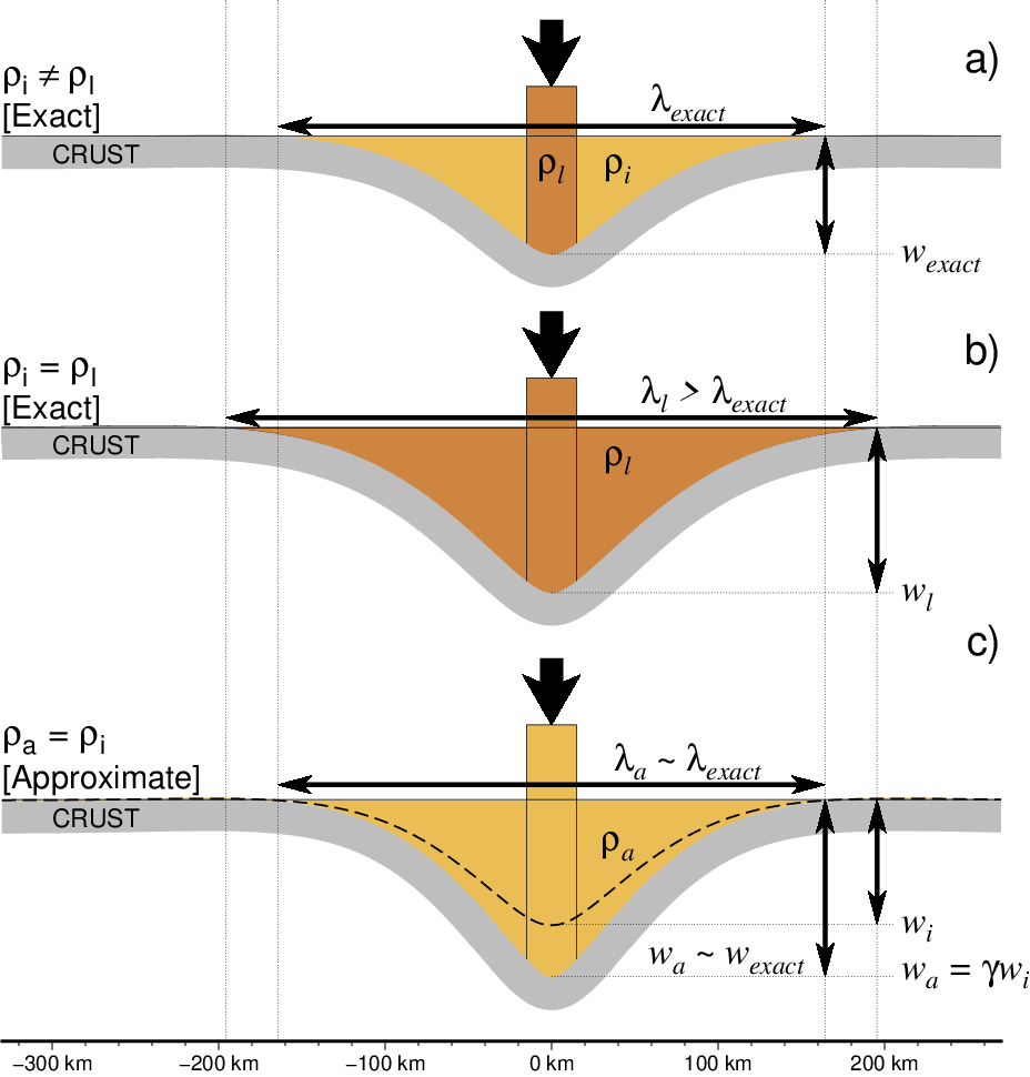
a) We want a flexural calculation that allows for different densities in the moat (\(\rho_i\)) and beneath the load (\(\rho_l\)). Unfortunately, the Fourier method requires a constant density contrast. b) Reusing the load density as a (higher) infill density gives an exact answer, but overestimates both the flexural wavelength (\(\lambda_l\)) and the amplitude of deflection (\(w_l\)). c) Reusing the infill density as a (lower) load density gives approximately the correct flexural wavelength but underestimates the amplitude (dashed curve). We achieve a satisfactory approximation by scaling \(w_i\) by the factor \(\gamma\) (modified from Wessel [2016]).
Elastic response function
The time-independent elastic response function is
where the flexural wavenumber k and constants \(\epsilon_s\) via in-plane stresses \(N_x, N_y, N_{xy}\) are
for subscripts \(s = \left (x, y, xy \right )\). In the most common scenario, \(N_s\) are all zero and the elastic response function becomes isotropic:
Firmoviscous response function
The firmoviscous response function \(\Phi(\mathbf{k},t)\) scales the magnitude of the deformation at a given wavenumber and time and depends on rheological parameters and in-plane stresses:
If the foundation is an inviscid half-space, then the relaxation parameter \(\tau(k_r) = \infty\), there is no time-dependence, and \(\Phi_{fv}(\mathbf{k},t) = \Phi_e(\mathbf{k})\). Otherwise, it is given by
where \(\beta(k_r)\) depends on whether we have a finite-thickness layer of thickness \(T_a\) and viscosity \(\eta_a\) above the half-space of viscosity \(\eta_m\) (Cathles, 1975; Nakada, 1986). If no finite layer exists then \(\beta(k_r) = 1\), otherwise
where
Airy and viscous response function
In the limit \(t \rightarrow \infty, \tau \rightarrow 0\) and we approach the purely elastic solution
Otherwise, if the plate has no strength (-E0), then \(\Phi_e(\mathbf{k}) = 1\) and the response function is purely viscous and isotropic:
For \(t \rightarrow \infty\) (or for an inviscid half-space) we approach Airy isostasy: \(w(\mathbf{x}) = A h(\mathbf{x})\).
Maxwell viscoelastic response
For case (4), the viscoelastic response function (only available for an inviscid substratum) is
where \(t_m\) is the Maxwell relaxation time (Watts, 2001).
General linear viscoelastic response
For case (5), the general linear viscoelastic response function (with an inviscid substratum) is (Karner, 1982)
where subscripts i and f refers to the initial (t = 0) and final (\(t = \infty\)) values for rigidities (\(D_i, D_f\)) and elastic response functions (\(\Phi_i, \Phi_f\)).
References
Cathles, L. M., 1975, The viscosity of the earth’s mantle, Princeton University Press.
Karner, G. D., 1982, Spectral representation of isostatic models, BMR J. Australian Geology & Geophysics, 7, 55-62.
Nakada, M., 1986, Holocene sea levels in oceanic islands: Implications for the rheological structure of the Earth’s mantle, Tectonophysics, 121, 263–276, http://dx.doi.org/10.1016/0040-1951(86)90047-8.
Watts, A. B., 2001, Isostasy and Flexure of the Lithosphere, 458 pp., Cambridge University Press.
Wessel. P., 2001, Global distribution of seamounts inferred from gridded Geosat/ERS-1 altimetry, J. Geophys. Res., 106(B9), 19,431-19,441, http://dx.doi.org/10.1029/2000JB000083.
Wessel, P., 2016, Regional–residual separation of bathymetry and revised estimates of Hawaii plume flux, Geophys. J. Int., 204(2), 932-947, http://dx.doi.org/10.1093/gji/ggv472.
See Also
gmt, gmtflexure, grdfft, gravfft grdmath, grdproject, grdseamount