grdseamount
Create synthetic seamounts (Gaussian, parabolic, polynomial, cone or disc; circular or elliptical)
Synopsis
gmt grdseamount [ table ] -Goutgrid -Iincrement -Rregion [ -A[out/in] ] [ -C[c|d|g|o|p] ] [ -Dunit ] [ -E ] [ -F[flattening] ] [ -L[cut] ] [ -M[list] ] [ -Nnorm ] [ -Qbmode/fmode[+d] ] [ -Sscale ] [ -Tt0[/t1/dt][+l] ] [ -Zlevel ] [ -V[level] ] [ -bibinary ] [ -eregexp ] [ -fflags ] [ -iflags ] [ -rreg ] [ --PAR=value ]
Note: No space is allowed between the option flag and the associated arguments.
Description
grdseamount will compute the combined shape of multiple synthetic seamounts given their individual shape parameters. We read from table (or stdin) a list of seamount locations and sizes and can evaluate either Gaussian, parabolic, conical, polynomial or disc shapes, which may be circular or elliptical, and optionally truncated. Various scaling options are available to modify the result, including an option to add in a background depth (more complicated backgrounds may be added via grdmath). The input data must contain lon, lat, radius, height for each seamount. For elliptical features (-E) we expect lon, lat, azimuth, semi-major, semi-minor, height instead. If flattening is specified (via -F) with no value appended then a final column with flattening is expected (cannot be used for plateaus). For temporal evolution of topography the -T option may be used, in which case the data file must have two final columns with the start and stop time of seamount construction. In this case you may choose to write out a cumulative shape or just the increments produced by each time step (see -Q). Finally, for mixing shapes you can use the trailing text to set the shape by using -C without an argument.
Required Arguments (if -L not given)
- table
One or more ASCII (or binary, see -bi[ncols][type]) data table file(s) holding a number of data columns. If no tables are given then we read from standard input.
-Goutgrid[=ID][+ddivisor][+ninvalid] [+ooffset|a][+sscale|a] [:driver[dataType][+coptions]]
Give the name of the output grid file. If -T is set then outgrid must be a filename template that contains a floating point format (C syntax). If the filename template also contains either %s (for unit name) or %c (for unit letter) then we use the corresponding time (in units specified in -T) to generate the individual file names, otherwise we use time in years with no unit. Optionally, append =ID for writing a specific file format (See full description). The following modifiers are supported:
+d - Divide data values by given divisor [Default is 1].
+n - Replace data values matching invalid with a NaN.
+o - Offset data values by the given offset, or append a for automatic range offset to preserve precision for integer grids [Default is 0].
+s - Scale data values by the given scale, or append a for automatic scaling to preserve precision for integer grids [Default is 1].
Note: Any offset is added before any scaling. +sa also sets +oa (unless overridden). To write specific formats via GDAL, use = gd and supply driver (and optionally dataType) and/or one or more concatenated GDAL -co options using +c. See the “Writing grids and images” cookbook section for more details.
- -Ix_inc[+e|n][/y_inc[+e|n]]
Set the grid spacing as x_inc [and optionally y_inc].
Geographical (degrees) coordinates: Optionally, append an increment unit. Choose among:
m to indicate arc minutes
s to indicate arc seconds
e (meter), f (foot), k (km), M (mile), n (nautical mile) or u (US survey foot), in which case the increment will be converted to the equivalent degrees longitude at the middle latitude of the region (the conversion depends on PROJ_ELLIPSOID). If y_inc is given but set to 0 it will be reset equal to x_inc; otherwise it will be converted to degrees latitude.
All coordinates: The following modifiers are supported:
+e to slightly adjust the max x (east) or y (north) to fit exactly the given increment if needed [Default is to slightly adjust the increment to fit the given domain].
+n to define the number of nodes rather than the increment, in which case the increment is recalculated from the number of nodes, the registration (see GMT File Formats), and the domain. Note: If -Rgrdfile is used then the grid spacing and the registration have already been initialized; use -I and -R to override these values.
- -Rxmin/xmax/ymin/ymax[+r][+uunit]
Specify the region of interest. (See full description) (See cookbook information).
Optional Arguments
- -A[out/in]
Build a mask grid, append outside/inside values [1/NaN]. Here, height and flattening are ignored and -L, -N and -Z are disallowed.
- -C[c|d|g|o|p]
Select seamount shape function: choose among c (cone), d (disc), g (Gaussian) o (polynomial) and p (parabolic) shape [Default is Gaussian]. All but the disc can furthermore be truncated via a flattening parameter f set by -F. If -C is not given any argument then we will read the shape code from the last input column. If -C is not given at all then we default to Gaussian shapes [g]. Note: The polynomial model has an amplitude for a normalized radius r that is given by \(h(r) = \frac{(1+r)^3(1-r)^3)}{1+r^3}\). It is very similar to the Gaussian model (volume is just ~2.4% larger) but h goes exactly to zero at the basal radius.
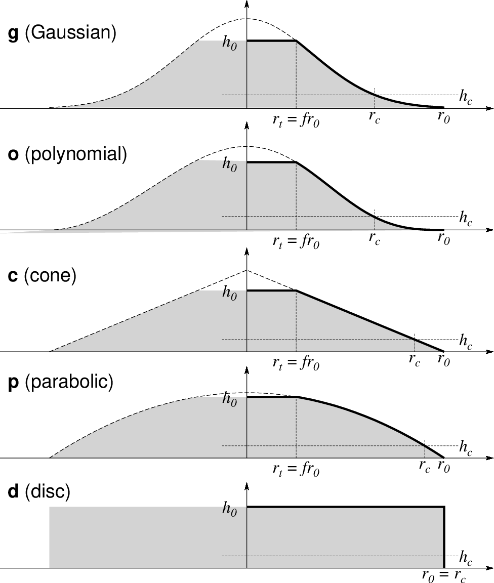
The five types of seamounts selectable via option -C. In all cases, \(h_0\) is the maximum height, \(r_0\) is the basal radius, \(h_c\) is the noise floor set via -L [0], and f is the flattening set via -F [0]. The top radius \(r_t\) is only nonzero if there is flattening and hence does not apply to the disc model.
- -Dunit
Append the unit used for horizontal distances in the input file (see Units). Does not apply for geographic data (-fflags) which we convert to km.
- -E
Elliptical data format. We expect the input records to contain lon, lat, azimuth, major, minor, height (with the latter in m) for each seamount. [Default is Circular data format, expecting lon, lat, radius, height].
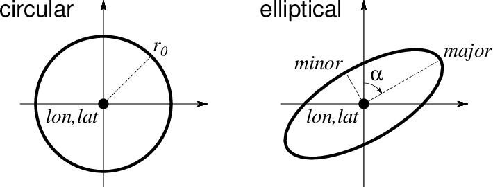
Use -E to select elliptical rather than circular shape in map view. Both shapes require lon, lat. Circular only requires the radius \(r_0\) while elliptical requires the azimuth \(\alpha\) and the major and minor semi-axes .
- -F[flattening]
Seamounts are to be truncated to guyots. Append flattening from 0 (no flattening) to 1 (no feature!), otherwise we expect to find it in last input column [no truncation]. Ignored if used with -Cd.
- -L[cut]
List area, volume, and mean height for each seamount; No grid is created. Optionally, append the noise-floor cutoff level below which we ignore area and volume [0].
- -M[list]
Write the times and names of all grids that were created to the text file list. Requires -T. If not list file is given then we write to standard output.
- -Nnorm
Normalize grid so maximum grid height equals norm [no normalization]
- -Qbmode/fmode[+d]
Only to be used in conjunction with -T. Append two different modes settings: The bmode determines how we construct the surface. Specify c for cumulative volume through time [Default], or i for incremental volume added for each time slice. The fmode determines the volume flux curve we use. Give c for a constant volume flux or g for a Gaussian volume flux [Default] between the start and stop times of each feature. These fluxes integrate to a linear or error-function volume fraction over time, respectively, as shown below. By default we compute the exact cumulative and incremental values for the seamounts specified. Append +d to instead approximate each incremental layer by a disc of constant thickness.
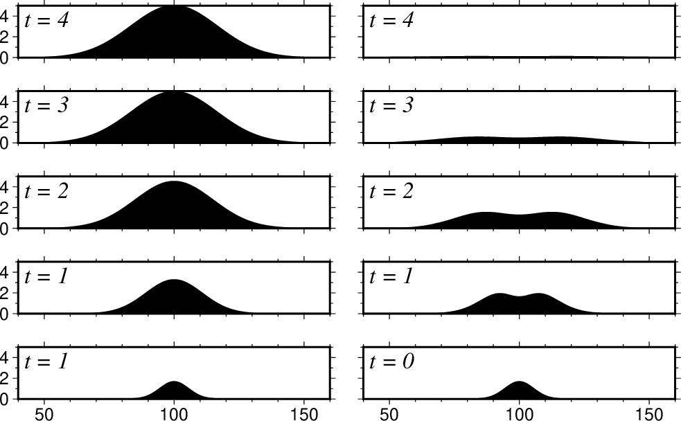
Use bmode in -Q to choose between cumulative output (c; actual topography as function of time [left]) or incremental output (i; the difference in actual topography over five time-steps [right]). Here we used -Cg for a Gaussian model with no flattening and a linear volume flux.
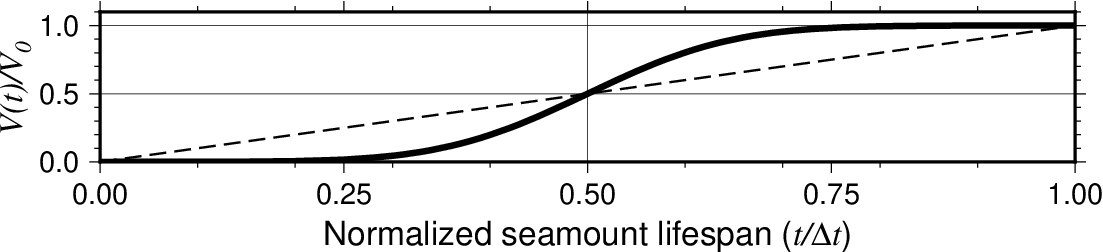
Use fmode in -Q to choose between a constant (c; dashed line) or Gaussian (g; heavy line) volume flux model.
- -Sscale
Sets optional scale factor for radii [1].
- -Tt0[/t1/dt][+l]
Specify t0, t1, and time increment (dt) for sequence of calculations [Default is one step, with no time dependency]. For a single specific time, just give start time t0. Default unit is years; append k for kyr and M for Myr. For a logarithmic time scale, append +l and specify n steps instead of dt. Alternatively, give a file with the desired times in the first column (these times may have individual units appended, otherwise we assume year). Note that a grid will be written for all time-steps even if there are no loads or no changes.
- -V[level]
Select verbosity level [w]. (See full description) (See cookbook information).
- -Zlevel
Set the background depth [0].
- -birecord[+b|l] (more …)
Select native binary format for primary table input. [Default is 4 input columns].
- -e[~]“pattern” | -e[~]/regexp/[i] (more …)
Only accept data records that match the given pattern.
- -fflags
Geographic grids (dimensions of longitude, latitude) will be converted to km via a “Flat Earth” approximation using the current ellipsoid parameters.
- -h[i|o][n][+c][+d][+msegheader][+rremark][+ttitle] (more …)
Skip or produce header record(s). Not used with binary data.
- -icols[+l][+ddivisor][+sscale|d|k][+ooffset][,…][,t[word]] (more …)
Select input columns and transformations (0 is first column, t is trailing text, append word to read one word only).
- -r[g|p] (more …)
Set node registration [gridline].
- -:[i|o] (more …)
Swap 1st and 2nd column on input and/or output.
- -^ or just -
Print a short message about the syntax of the command, then exit (NOTE: on Windows just use -).
- -+ or just +
Print an extensive usage (help) message, including the explanation of any module-specific option (but not the GMT common options), then exit.
- -? or no arguments
Print a complete usage (help) message, including the explanation of all options, then exit.
- --PAR=value
Temporarily override a GMT default setting; repeatable. See gmt.conf for parameters.
Units
For map distance unit, append unit d for arc degree, m for arc minute, and s for arc second, or e for meter [Default], f for foot, k for km, M for statute mile, n for nautical mile, and u for US survey foot. By default we compute such distances using a spherical approximation with great circles (-jg) using the authalic radius (see PROJ_MEAN_RADIUS). You can use -jf to perform “Flat Earth” calculations (quicker but less accurate) or -je to perform exact geodesic calculations (slower but more accurate; see PROJ_GEODESIC for method used).
Examples
To compute the incremental loads from two elliptical, truncated Gaussian seamounts being constructed from 3 Ma to 2 Ma and 2.8 M to 1.9 Ma using a constant volumetric production rate, and output an incremental grid every 0.1 Myr from 3 Ma to 1.9 Ma, we can try:
cat << EOF > t.txt
#lon lat azimuth, semi-major, semi-minor, height tstart tend
0   0       -20     120     60      5000    3.0M    2M
50  80      -40     110     50      4000    2.8M    21.9M
EOF
gmt grdseamount -Rk-1024/1022/-1122/924 -I2000 -Gsmt_%3.1f_%s.nc t.txt -T3M/1.9M/0.1M -Qi/c -Dk -E -F0.2 -Cg -Ml.lis
The file l.lis will contain records with numerical time, gridfile, and unit time.