binstats
Bin spatial data and determine statistics per bin
Synopsis
gmt binstats [ table ] -Goutgrid -Iincrement -Ca|d|g|i|l|L|m|n|o|p|q[quant]|r|s|u|U|z -Rregion -Sradius [ -Eempty ] [ -N ] [ -T[h|r] ] [ -V[level] ] [ -W[+s] ] [ -aflags ] [ -bibinary ] [ -dinodata[+ccol] ] [ -eregexp ] [ -fflags ] [ -ggaps ] [ -hheaders ] [ -iflags ] [ -qiflags ] [ -rreg ] [ -wflags ] [ -:[i|o] ] [ --PAR=value ]
Note: No space is allowed between the option flag and the associated arguments.
Description
binstats reads arbitrarily located (x, y[, z][, w]) points (2-4 columns) from standard input [or table] and for each node in the specified grid layout determines which points are within the given radius. These points are then used in the calculation of the specified statistic. The results may be presented as is or may be normalized by the circle area to perhaps give density estimates. Alternatively, select hexagonal tiling instead or a rectangular grid layout.
Required Arguments
- table
A 2-4 column ASCII file(s) [or binary, see -bi] holding (x, y[, z][, w]) data values. You must use -W to indicate that you have weights. Only -Cn will accept 2 columns only. If no file is specified, binstats will read from standard input.
- -Ca|d|g|i|l|L|m|n|o|p|q[quant]|r|s|u|U|z
Choose the statistic that will be computed per node based on the points that are within radius distance of the node. Append one directive among these candidates:
a: Mean (i.e., average).
d: Median absolute deviation (MAD).
g: The full (max-min) range.
i: The 25-75% interquartile range.
l: Minimum (lowest value).
L: Minimum of positive values only.
m: Median value.
n: The number of values per bin.
o: Least median square (LMS) scale.
p: Mode (maximum likelihood estimate).
q: Selected quantile (append desired quantile in 0-100% range [50]).
r: Root mean square (RMS).
s: Standard deviation.
u: Maximum (highest value).
U: Maximum of negative values only.
z: The sum of the values.
-Goutgrid[=ID][+ddivisor][+ninvalid][+ooffset|a][+sscale|a][:driver[dataType][+coptions]]
Optionally, append =ID for writing a specific file format. The following modifiers are supported:
+d - Divide data values by given divisor [Default is 1].
+n - Replace data values matching invalid with a NaN.
+o - Offset data values by the given offset, or append a for automatic range offset to preserve precision for integer grids [Default is 0].
+s - Scale data values by the given scale, or append a for automatic scaling to preserve precision for integer grids [Default is 1].
Note: Any offset is added before any scaling. +sa also sets +oa (unless overridden). To write specific formats via GDAL, use =gd and supply driver (and optionally dataType) and/or one or more concatenated GDAL -co options using +c. See the “Writing grids and images” cookbook section for more details.
- -Ix_inc[+e|n][/y_inc[+e|n]]
Set the grid spacing as x_inc [and optionally y_inc].
Geographical (degrees) coordinates: Optionally, append an increment unit. Choose among:
d - Indicate arc degrees
m - Indicate arc minutes
s - Indicate arc seconds
If one of e (meter), f (foot), k (km), M (mile), n (nautical mile) or u (US survey foot), the increment will be converted to the equivalent degrees longitude at the middle latitude of the region (the conversion depends on PROJ_ELLIPSOID). If y_inc is not given or given but set to 0 it will be reset equal to x_inc; otherwise it will be converted to degrees latitude.
All coordinates: The following modifiers are supported:
+e - Slightly adjust the max x (east) or y (north) to fit exactly the given increment if needed [Default is to slightly adjust the increment to fit the given domain].
+n - Define the number of nodes rather than the increment, in which case the increment is recalculated from the number of nodes, the registration (see GMT File Formats), and the domain. Note: If -Rgrdfile is used then the grid spacing and the registration have already been initialized; use -I and -R to override these values.
- -Rxmin/xmax/ymin/ymax[+r][+uunit]
Specify the region of interest. (See full description) (See technical reference).
Optional Arguments
- -Eempty
Set the value assigned to empty nodes [NaN].
- -N
Normalize the resulting grid values by the area represented by the search radius [no normalization].
- -Sradius
Sets the search radius that determines which data points are considered close to a node. Append the distance unit (see Units). Not compatible with -T.
- -T[h|r]
Instead of circular, possibly overlapping areas, select non-overlapping tiling. Choose between rectangular and hexagonal binning. For -Tr, set bin sizes via -I and we write the computed statistics to the grid file named in -G. For -Th, we write a table with the centers of the hexagons and the computed statistics to standard output (or to the file named in -G). Here, the -I setting is expected to set the y increment only and we compute the x-increment given the geometry. Because the horizontal spacing between hexagon centers in x and y have a ratio of \(\sqrt{3}\), we will automatically adjust xmax in -R to fit a whole number of hexagons. Note: Hexagonal tiling requires Cartesian data.
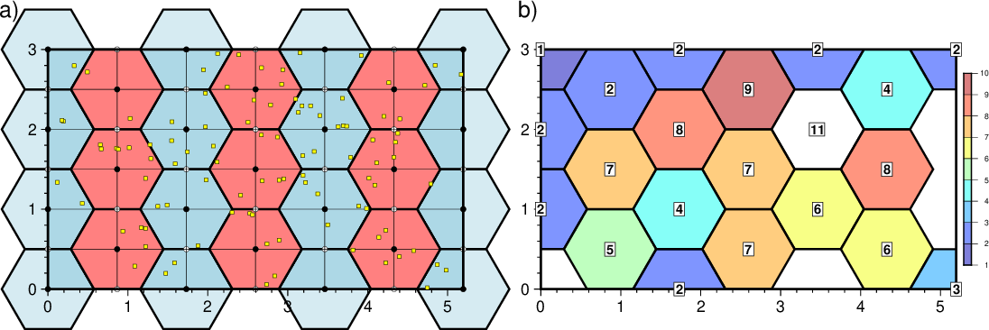
a) Hexagonal polygons (light blue and light red) used for binning. The red are all inside the gridding region while the blue are outside along the border. Yellow squares are test data, black nodes are grid nodes supported by a hexagon center, and while squares are nodes that fall between. b) Grid showing result of hexagonal binning which yields a constant value inside each polygon.
- -V[level]
Select verbosity level [w]. (See full description) (See technical reference).
- -W[+s]
Input data have an extra column containing observation point weight. If weights are given then weighted statistical quantities will be computed while the count will be the sum of the weights instead of number of points. If your weights are actually uncertainties (\(1\sigma\)) then append +s and we compute weight = \(\frac{1}{\sigma}\).
- -a[[col=]name[,…]] (more …)
Set aspatial column associations col=name.
- -birecord[+b|l] (more …)
Select native binary format for primary table input. [Default is 3 (or 4 if -W is set) columns].
- -dinodata[+ccol] (more …)
Replace input columns that equal nodata with NaN.
- -e[~]“pattern” | -e[~]/regexp/[i] (more …)
Only accept data records that match the given pattern.
- -f[i|o]colinfo (more …)
Specify data types of input and/or output columns.
- -gx|y|z|d|X|Y|Dgap[u][+a][+ccol][+n|p] (more …)
Determine data gaps and line breaks.
- -h[i|o][n][+c][+d][+msegheader][+rremark][+ttitle] (more …)
Skip or produce header record(s).
- -icols[+l][+ddivisor][+sscale|d|k][+ooffset][,…][,t[word]] (more …)
Select input columns and transformations (0 is first column, t is trailing text, append word to read one word only).
- -qi[~]rows|limits[+ccol][+a|t|s] (more …)
Select input rows or data limit(s) [default is all rows].
- -r[g|p] (more …)
Set node registration [gridline].
- -wy|a|w|d|h|m|s|cperiod[/phase][+ccol] (more …)
Convert an input coordinate to a cyclical coordinate.
- -:[i|o] (more …)
Swap 1st and 2nd column on input and/or output.
- -^ or just -
Print a short message about the syntax of the command, then exit (Note: on Windows just use -).
- -+ or just +
Print an extensive usage (help) message, including the explanation of any module-specific option (but not the GMT common options), then exit.
- -? or no arguments
Print a complete usage (help) message, including the explanation of all options, then exit.
- --PAR=value
Temporarily override a GMT default setting; repeatable. See gmt.conf for parameters.
Units
For map distance unit, append unit d for arc degree, m for arc minute, and s for arc second, or e for meter [Default unless stated otherwise], f for foot, k for km, M for statute mile, n for nautical mile, and u for US survey foot. By default we compute such distances using a spherical approximation with great circles (-jg) using the authalic radius (see PROJ_MEAN_RADIUS). You can use -jf to perform “Flat Earth” calculations (quicker but less accurate) or -je to perform exact geodesic calculations (slower but more accurate; see PROJ_GEODESIC for method used).
Grid Values Precision
Regardless of the precision of the input data, GMT programs that create grid files will internally hold the grids in 4-byte floating point arrays. This is done to conserve memory and furthermore most if not all real data can be stored using 4-byte floating point values. Data with higher precision (i.e., double precision values) will lose that precision once GMT operates on the grid or writes out new grids. To limit loss of precision when processing data you should always consider normalizing the data prior to processing.
Examples
Note: Below are some examples of valid syntax for this module.
The examples that use remote files (file names starting with @)
can be cut and pasted into your terminal for testing.
Other commands requiring input files are just dummy examples of the types
of uses that are common but cannot be run verbatim as written.
To examine the population inside a circle of 1000 km radius for all nodes in a 5x5 arc degree grid, using the remote file @capitals.gmt, and plot the resulting grid using default projection and colors, try:
gmt begin map
  gmt binstats @capitals.gmt -a2=population -Rg -I5 -Cz -Gpop.nc -S1000k
  gmt grdimage pop.nc -B
gmt end show
To do hexagonal binning of the data in the file mydata.txt and counting the number of points inside each hexagon, try:
gmt binstats mydata.txt -R0/5/0/3 -I1 -Th -Cn > counts.txt
See Also
blockmean, blockmedian, blockmode, gmt, nearneighbor, triangulate, xyz2grd