(50) Probability distributions
This example presents visually the various probability distributions available in gmtmath (as well as grdmath). We evaluate and display both the probability density function (pdf) and the cumulative distribution function (cdf) for each case. The left column shows the density functions while the right column shows the cumulative functions. In addition to the distributions you can also use gmtmath to evaluate critical values for the distributions for chosen confidence levels.
#!/usr/bin/env bash
#               GMT EXAMPLE 50
#
# Purpose:      Illustrate different statistical distributions in gmtmath
# GMT modules:  math, set, plot, text
# Unix progs:	rm
#

gmt begin ex50
	# Left column have all the PDFs
	# Binomial distribution
	gmt math -T0/8/1 0.25 8 T BPDF = p.txt
	gmt plot -R-0.6/8.6/0/0.35 -JX7.5c/1.25c -Glightgreen p.txt -Sb0.8q -W0.5p -BWS -Bxa1 -Byaf
	# Poisson distribution
	gmt math -T0/8/1 T 2 PPDF = p.txt
	gmt plot -R-0.6/8.6/0/0.3 -Glightgreen p.txt -Sb0.8q -W0.5p -BWS -Bxa1 -Byaf -Y2.25c
	# Plot normal distribution
	gmt math -T-4/4/0.1 T ZPDF = p.txt
	gmt plot -R-4/4/0/0.4 p.txt -L+yb -Glightgreen -W1p -BWS -Bxa1 -Byaf -Y2.25c
	# Plot t distribution
	gmt plot -R-4/4/0/0.4 p.txt -W1p,lightgray -Y2.25c
	gmt math -T-4/4/0.1 T 3 TPDF = p.txt
	gmt plot p.txt -L+yb -Glightgreen -W1p -BWS -Bxa1 -Byaf
	# Plot F distribution
	gmt math -T0/6/0.02 T 20 12 FPDF = p.txt
	gmt plot -R0/6/0/1.02 p.txt -L+yb -Glightgreen -W1p -BWS -Bxa1 -Byaf -Y2.25c
	# Plot Laplace distribution
	gmt math -T-4/4/0.1 T LPDF = p.txt
	gmt plot -R-4/4/0/0.5 p.txt -L+yb -Glightgreen -W1p -BWS -Bxa1 -Byaf -Y2.25c
	# Plot Exponential distribution
	gmt math -T0/4/0.1 T 2 EPDF = p.txt
	gmt plot -R0/4/0/2.0 p.txt -L+yb -Glightgreen -W1p -BWS -Bxa1 -Byaf -Y2.25c
	# Plot Rayleigh distribution
	gmt math -T0/6/0.1 T RPDF = p.txt
	gmt plot -R0/6/0/0.7 p.txt -L+yb -Glightgreen -W1p -BWS -Bxa1 -Byaf -Y2.25c
	# Plot Weibull distribution
	gmt math -T0/6/0.1 T 1 1.5 WPDF = p.txt
	gmt plot -R0/6/0/0.8 p.txt -L+yb -Glightgreen -W1p -BWS -Bxa1 -Byaf -Y2.25c
	# Plot Chi-squared distribution
	gmt math -T0/12/0.1 T 4 CHI2PDF = p.txt
	gmt plot -R0/12/0/0.20 p.txt -L+yb -Glightgreen -W1p -BWS -Bxa1 -Byaf -Y2.25c
	# Right column has all the CDF
	# Plot binomial cumulative distribution
	gmt math -T0/8/1 0.25 8 T BCDF = p.txt
	gmt plot -R-0.6/8.6/0/1.02 -Glightred p.txt -Sb0.8q -W0.5p -BES -Bxa1 -Byaf -X9c -Y-8.1i
	# Plot Poisson cumulative distribution
	gmt math -T0/8/1 T 2 PCDF = p.txt
	gmt plot -R-0.6/8.6/0/1.02 -Glightred p.txt -Sb0.8q -W0.5p -BES -Bxa1 -Byaf -Y2.25c
	# Plot normal cumulative distribution
	gmt math -T-4/4/0.1 T ZCDF = p.txt
	gmt plot -R-4/4/0/1.02 p.txt -L+yb -Glightred -W1p -BES -Bxa1 -Byaf -Y2.25c
	# Plot t cumulative distribution
	gmt plot -R-4/4/0/1.02 p.txt -W1p,lightgray -Y2.25c
	gmt math -T-4/4/0.1 T 3 TCDF = p.txt
	gmt plot p.txt -L+yb -Glightred -W1p -BES -Bxa1 -Byaf
	# Plot F cumulative distribution
	gmt math -T0/6/0.02 T 20 12 FCDF = p.txt
	gmt plot -R0/6/0/1.02 p.txt -L+yb -Glightred -W1p -BES -Bxa1 -Byaf -Y2.25c
	# Plot Laplace cumulative distribution
	gmt math -T-4/4/0.1 T LCDF = p.txt
	gmt plot -R-4/4/0/1.02  p.txt -L+yb -Glightred -W1p -BES -Bxa1 -Byaf -Y2.25c
	# Plot Exponential cumulative distribution
	gmt math -T0/4/0.1 T 2 ECDF = p.txt
	gmt plot -R0/4/0/1.02 p.txt -L+yb -Glightred -W1p -BES -Bxa1 -Byaf -Y2.25c
	# Plot Rayleigh cumulative distribution
	gmt math -T0/6/0.1 T RCDF = p.txt
	gmt plot -R0/6/0/1.02 p.txt -L+yb -Glightred -W1p -BES -Bxa1 -Byaf -Y2.25c
	# Plot Weibull cumulative distribution
	gmt math -T0/6/0.1 T 1 1.5 WCDF = p.txt
	gmt plot -R0/6/0/1.02 p.txt -L+yb -Glightred -W1p -BES -Bxa1 -Byaf -Y2.25c
	# Plot Chi-squared cumulative distribution
	gmt math -T0/12/0.1 T 4 CHI2CDF = p.txt
	gmt plot -R0/12/0/1.02 p.txt -L+yb -Glightred -W1p -BES -Bxa1 -Byaf -Y2.25c
	gmt text -R0/17/0/3 -Jx1c -N -X-9c -F+f18p+cTC+t"Probability @;lightgreen;Density@;; and @;lightred;Cumulative@;; Distribution Functions"
	gmt text -R0/17/0/25 -F+f14p,Times-Italic+jTC -Dj0.9c -N -Y-20.25c <<- EOF
	8.3  2.25 Binomial P@-8,0.25@-
	8.3  4.50 Poisson P(@~l=2@~)
	8.3  6.75 Normal P(z)
	8.3  9.00 Student t(@~n=3@~)
	8.3 11.25 F(@~n@-1@-=20, n@-2@- = 12@~)
	8.3 13.50 Laplace P(z)
	8.3 15.75 Exponential P(@~l=2@~)
	8.3 18.00 Rayleigh P(z)
	8.3 20.25 Weibull P(z,1,1.5)
	8.3 22.50 @~c@~@+2@+(z,@~n=4@~)
	EOF
	rm -f p.txt
gmt end show
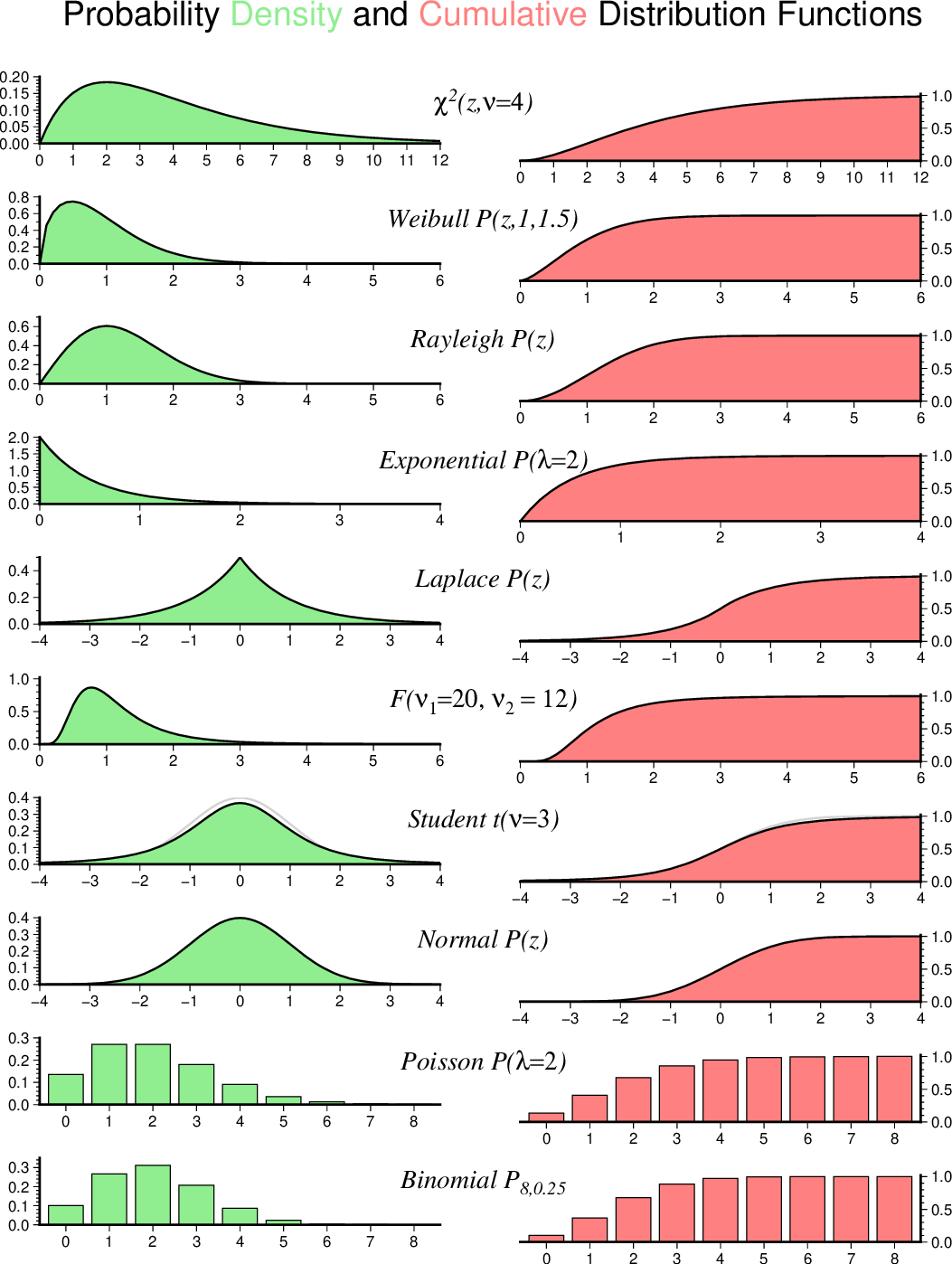
Probability distributions.