(36) Spherical gridding using Renka’s algorithms
The next script produces the plot in Figure. Here we demonstrate how sphinterpolate can be used to perform spherical gridding. Our example uses early measurements of the radius of Mars from Mariner 9 and Viking Orbiter spacecrafts. The middle panels shows the data distribution while the top and bottom panel are images of the interpolation using a piecewise linear interpolation and a smoothed spline interpolation, respectively. For spherical gridding with large volumes of data we recommend sphinterpolate while for small data sets (such as this one, actually) you have more flexibility with greenspline.
#!/usr/bin/env bash
#               GMT EXAMPLE 36
#
# Purpose:      Illustrate sphinterpolate with Mars radii data
# GMT modules:  plot, makecpt, grdimage, sphinterpolate, subplot
# Unix progs:   rm
#
gmt begin ex36
	# Interpolate data of Mars radius from Mariner9 and Viking Orbiter spacecrafts
	gmt subplot begin 3x1 -Fs14c/0 -JH0/14c -Rg -M0
		gmt makecpt -Crainbow -T-7000/15000
		# Piecewise linear interpolation; no tension
		gmt sphinterpolate @mars370d.txt -Rg -I1 -Q0 -Gtt.nc
		gmt grdimage tt.nc -Bag -c0

		gmt plot @mars370d.txt -Sc0.1c -G0 -B30g30 -c1

		# Smoothing
		gmt sphinterpolate @mars370d.txt -Rg -I1 -Q3 -Gtt.nc
		gmt grdimage tt.nc -Bag -c2
	gmt subplot end
	# cleanup
	rm -f tt.nc
gmt end show
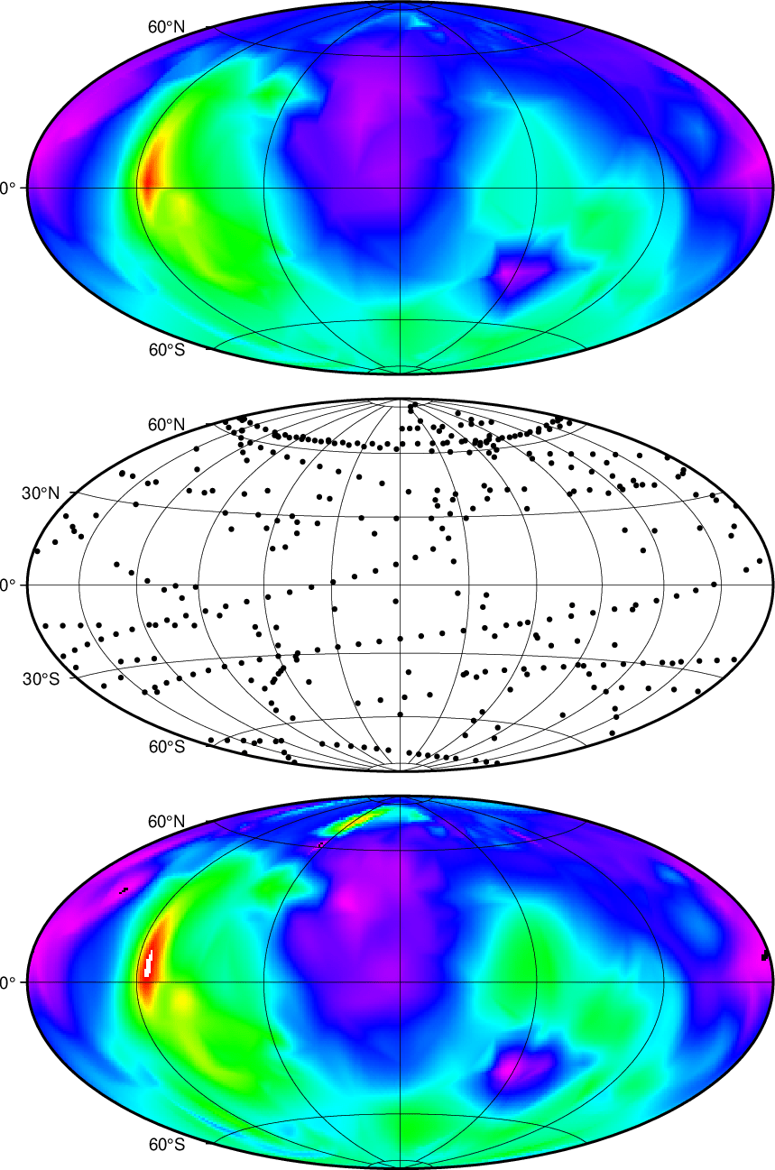
Spherical gridding using Renka's algorithms.