(16) Gridding of data, continued
contour (for contouring) and triangulate (for gridding) use the simplest method of interpolating data: a Delaunay triangulation (see Example (12) Optimal triangulation of data) which forms z(x, y) as a union of planar triangular facets. One advantage of this method is that it will not extrapolate z(x, y) beyond the convex hull of the input (x, y) data. Another is that it will not estimate a z value above or below the local bounds on any triangle. A disadvantage is that the z(x, y) surface is not differentiable, but has sharp kinks at triangle edges and thus also along contours. This may not look physically reasonable, but it can be filtered later (last panel below). surface can be used to generate a higher-order (smooth and differentiable) interpolation of z(x, y) onto a grid, after which the grid may be illustrated (grdcontour, grdimage, grdview). surface will interpolate to all (x, y) points in a rectangular region, and thus will extrapolate beyond the convex hull of the data. However, this can be masked out in various ways (see Example (15) Gridding, contouring, and masking of unconstrained areas).
A more serious objection is that surface may estimate z values outside the local range of the data (note area near x = 0.8, y = 5.3). This commonly happens when the default tension value of zero is used to create a “minimum curvature” (most smooth) interpolant. surface can be used with non-zero tension to partially overcome this problem. The limiting value tension = 1 should approximate the triangulation, while a value between 0 and 1 may yield a good compromise between the above two cases. A value of 0.5 is shown in the Figure More ways to grid data. A side effect of the tension is that it tends to make the contours turn near the edges of the domain so that they approach the edge from a perpendicular direction. A solution is to use surface in a larger area and then use grdcut to cut out the desired smaller area. Another way to achieve a compromise is to interpolate the data to a grid and then filter the grid using grdfft or grdfilter. The latter can handle grids containing “NaN” values and it can do median and mode filters as well as convolutions. Shown here is triangulate followed by grdfilter. Note that the filter has done some extrapolation beyond the convex hull of the original x, y values. The “best” smooth approximation of z(x, y) depends on the errors in the data and the physical laws obeyed by z. GMT cannot always do the “best” thing but it offers great flexibility through its combinations of tools. We illustrate all four solutions using a CPT that contains color fills, predefined patterns for interval (900,925) and NaN, an image pattern for interval (875,900), and a “skip slice” request for interval (700,725). Again, we use subplot to set up and place the four panels, and place the colorbar beneath the subplot.
#!/usr/bin/env bash
#		GMT EXAMPLE 16
#
# Purpose:	Illustrates interpolation methods using same data as Example 12.
# GMT modules:	gmtset, grdview, grdfilter, contour, colorbar, surface, triangulate
# Unix progs:	rm
#
gmt begin ex16
	gmt subplot begin 2x2 -M0.1c -Fs8c/0 -R-0.2/6.6/-0.2/6.6 -Jx1c -Scb -Srl+t -Bwesn -T"Gridding of Data"
		gmt surface @Table_5_11.txt -I0.2 -Graws0.nc
		gmt contour @Table_5_11.txt -C@ex_16.cpt -I -B+t"contour (triangulate)" -c0,0
		#
		gmt grdview raws0.nc -C@ex_16.cpt -Qs -B+t"surface (tension = 0)" -c0,1
		#
		gmt surface @Table_5_11.txt -Graws5.nc -T0.5
		gmt grdview raws5.nc -C@ex_16.cpt -Qs -B+t"surface (tension = 0.5)" -c1,0
		#
		gmt triangulate @Table_5_11.txt -Grawt.nc
		gmt grdfilter rawt.nc -Gfiltered.nc -D0 -Fc1
		gmt grdview filtered.nc -C@ex_16.cpt -Qs -B+t"triangulate @~\256@~ grdfilter" -c1,1
	gmt subplot end
	gmt colorbar -DJBC -C@ex_16.cpt
gmt end show
rm -f raws0.nc raws5.nc rawt.nc filtered.nc
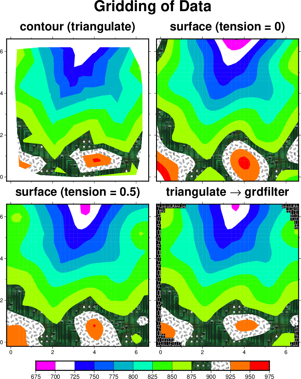
More ways to grid data