(49) Analysis of the Atlantic seafloor depth/age relationship

In this example we show an example of data analysis using grids of seafloor depth and age for a region in the south Atlantic. Dumping separate x,y,z triplets with grd2xyz lets us paste the output back via gmtconvert to make binary tables of age,depth,depth. Here, depth is repeated in order to use blockmode for modal depth estimation and xyz2grd for mapping the data density. We image the density of (age,depth) points, overlay the modal depths and their robust uncertainty bars, and compute and plot two models for the expected depths as a function of age (see legend). Note we place most of the legend twice to achieve the thin-on-thick pen effect in the legend.

#!/usr/bin/env bash
#               GMT EXAMPLE 49
#
# Purpose:      Illustrate data analysis using the seafloor depth/age relationship
# GMT modules:  blockmode, gmtmath, grdcontour, grdimage, grdsample, makecpt,
#		subplot, basemap, legend, colorbar, plot, xyz2grd
#

gmt begin ex49
	# Pull depth and age subsets from the global remote files
	gmt grdcut @earth_relief_02m -R30W/5E/30S/5S -Gdepth_pixel.nc
	gmt grdcut @earth_age_02m -R30W/5E/30S/5S -Gage_pixel.nc
	# Flip to positive depths in km
	gmt grdmath depth_pixel.nc NEG 1000 DIV = depth_pixel.nc
	# Obtain depth, age pairs by dumping grids and pasting results
	gmt grd2xyz age_pixel.nc -bof > age.bin
	gmt grd2xyz depth_pixel.nc -bof > depth.bin
	gmt convert -A age.bin depth.bin -bi3f -o2,5,5 -bo3f > depth-age.bin
	# Obtain modal depths every ~5 Myr
	gmt blockmode -R0/100/0/10 -I5/10 -r -E -Q depth-age.bin -bi3f -o0,2,3 > modal.txt
	# Create density grid of (age,depth) distribution
	gmt xyz2grd -R0/100/0/6.5 -I0.25/0.025 -r depth-age.bin -bi3f -An -Gdensity.nc
	# Make CPTs for ages and depths
	gmt makecpt -Chot -T0/100/10 -H > t.cpt
	gmt makecpt -Cabyss -T0/7 -H -I > z.cpt
	gmt subplot begin 2x1 -Fs15c/11.3c -Sc
		# Image depth distribution, modal depths, and competing predictions
		gmt grdimage density.nc -Q -Ct.cpt -JX15c/-11.3c -Bxaf+u" Myr" -Byaf+u" km" -c
		# Compute Parsons & Sclater [1977] depth-age curve (in km)
		# depth(t) =   0.35 * sqrt(t) + 2.500, t < 70 Myr
		#	   =  6.4 - 3.2 exp (-t/62.8), t > 70 Myr
		gmt math -T0/100/0.1 T SQRT 0.35 MUL 2.5 ADD T 70 LE MUL 6.4 T 62.8 DIV NEG EXP 3.2 MUL SUB T 70 GT MUL ADD = ps.txt
		gmt plot ps.txt -W4p,green
		gmt plot ps.txt -W1p
		# Compute Stein & Stein [1992] depth-age curve (in km)
		# depth(t) =  0.365 * sqrt(t) + 2.6,  t < 20 Myr
		#	   = 5.651 - 2.473 * exp (-0.0278*t), t > 20 Myr
		gmt math -T0/100/0.1 T SQRT 0.365 MUL 2.6 ADD T 20 LE MUL 5.651 T -0.0278 MUL EXP 2.473 MUL SUB T 20 GT MUL ADD = ss.txt
		# Plot curves and place the legend
		gmt plot ss.txt -W4p,white
		gmt plot ss.txt -W1p
		gmt plot -Ss0.4c -Gblue modal.txt -Ey+p1p,blue
		gmt plot -Ss0.1c -Gwhite modal.txt
		gmt legend -DjRT+w5.5c+o0.25c -F+p1p+gbeige+s <<- EOF
		S 0.5c - 0.9c - 4p,green 1.2c Parsons & Sclater (1977)
		S 0.5c - 0.9c - 4p,white 1.2c Stein & Stein (1992)
		S 0.5c s 0.4c blue - 1.2c Modal depth estimates
		EOF
		gmt legend -DjRT+w5.5c+o0.25c <<- EOF
		S 0.5c - 0.9c - 1p 0.75c
		S 0.5c - 0.9c - 1p 0.75c
		S 0.5c s 0.1c white - 0.75c
		EOF
		# Image depths with color-coded age contours
		gmt grdimage depth_pixel.nc -R30W/5E/30S/5S -JM? -Cz.cpt -c
		gmt plot -W1p @ridge_49.txt
		gmt grdcontour age_pixel.nc -A+f14p -Ct.cpt -Wa0.1p+c -GL30W/22S/5E/13S
		gmt colorbar -Cz.cpt -DjTR+w4.7c/0.4c+h+r+o0.85c/0.35c -Baf+u" km" -F+p1p+gbeige+s+c0p/10p/4p/4p
	gmt subplot end
	rm -f age_pixel.nc depth_pixel.nc age.bin depth.bin depth-age.bin density.nc modal.txt ps.txt ss.txt z.cpt t.cpt
gmt end show

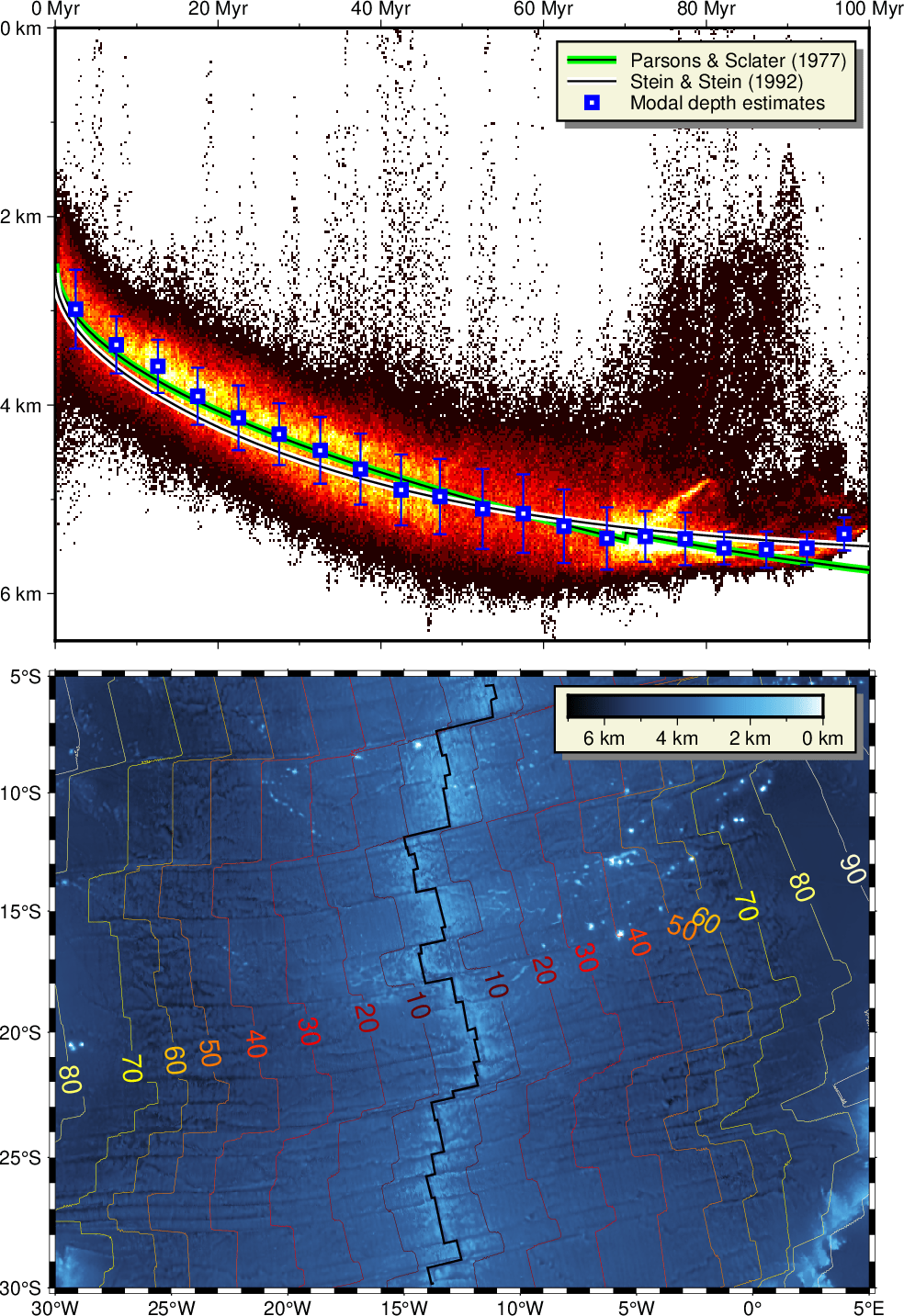
Seafloor depth vs. age in the south Atlantic.