Session Three
Contouring gridded data sets
GMT comes with several utilities that can create gridded data sets; we will discuss two such modules later this session. The data sets needed for this tutorial are obtained via the Internet as they are needed. Here, we will use grdcut to obtain and extract a GMT-ready grid that we will next use for contouring:
gmt grdcut @earth_relief_05m -R-66/-60/30/35 -Gtut_bathy.nc -V
Here we use the file extension .nc instead of the generic .grd to indicate that this is a netCDF file. It is good form, but not essential, to use .nc for netCDF grids. Using that extension will help other programs installed on your system to recognize these files and might give it an identifiable icon in your file browser. Learn about other programs that read netCDF files at the netCDF website. You can also obtain tut_bathy.nc from the GMT cache server as we are doing below. Feel free to open it in any other program and compare results with GMT.
We first use the GMT module grdinfo to see what’s in this file:
gmt grdinfo @tut_bathy.nc
The file contains bathymetry for the Bermuda region and has depth values from -5475 to -89 meters. We want to make a contour map of this data; this is a job for grdcontour. As with previous plot commands we need to set up the map projection with -J. Here, however, we do not have to specify the region since that is by default assumed to be the extent of the grid file. To generate any plot we will in addition need to supply information about which contours to draw. Unfortunately, grdcontour is a complicated module with too many options. We put a positive spin on this situation by touting its flexibility. Here are the most useful options:
Option
Purpose
-Aannot_int
Annotation interval and attributes
-Ccont_int
Contour interval
-Ggap
Controls placement of contour annotations
-Llow/high
Only draw contours within the low to high range
-Qcut
Do not draw contours with fewer than cut points
-Ssmooth
Resample contours smooth times per grid cell increment
-T[+|-][+dgap[/length]][+l[labels]]
Draw tick-marks in downhill
direction for innermost closed contours. Add tick spacing
and length, and characters to plot at the center of closed contours
-W[a|c]pen
Set contour and annotation pens
-Z[+sfactor][+ooffset]
Subtract offset and multiply data by factor prior to processing
We will first make a plain contour map using 1 km as annotation interval and 250 m as contour interval. We choose a 7-inch-wide Mercator plot and annotate the borders every 2°:
gmt begin GMT_tut_11
	gmt set GMT_THEME cookbook
	gmt grdcontour @earth_relief_05m -R-66/-60/30/35 -JM6i -C250 -A1000 -B
gmt end show
Your plot should look like our example 11 below
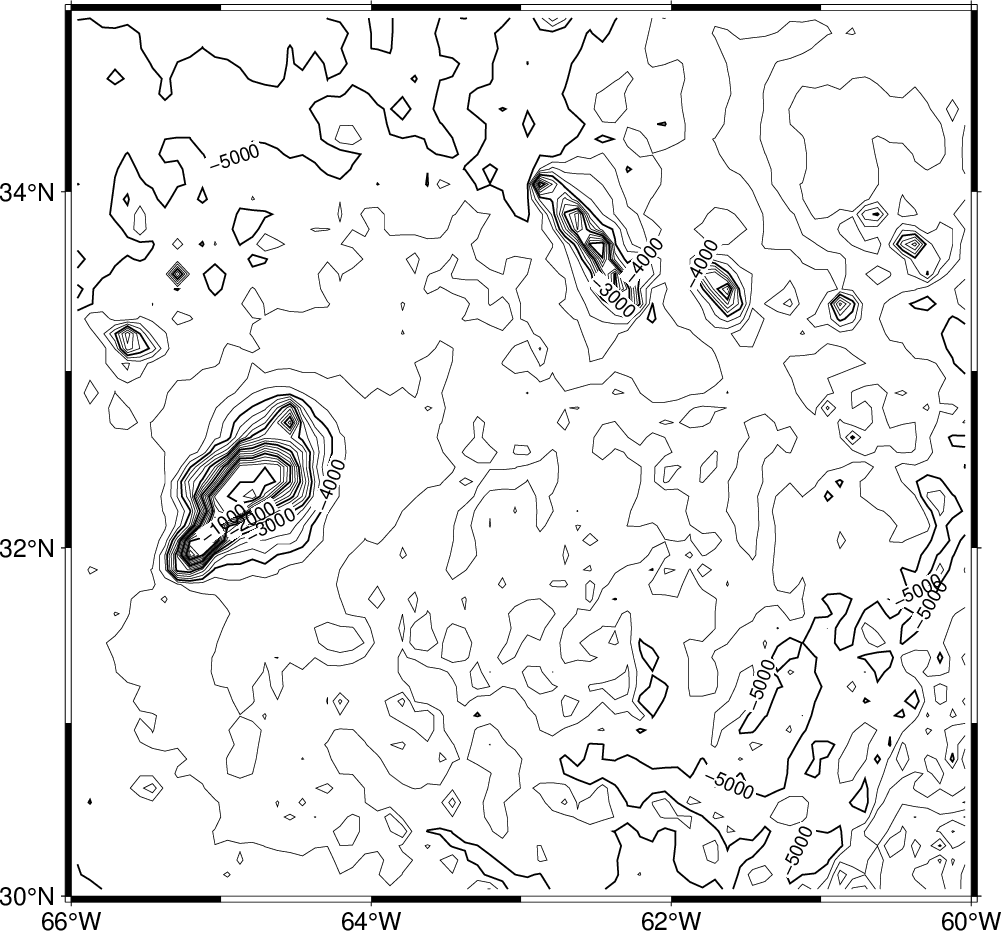
Result of GMT Tutorial example 11
Exercises:
Add smoothing with -S4.
Try tick all highs and lows with -T.
Skip small features with -Q10.
Override region using -R-70/-60/25/35.
Try another region that clips our data domain.
Scale data to km and use the km unit in the annotations.
Gridding of arbitrarily spaced data
Except in the situation above when a grid file is available, we must convert our data to the right format readable by GMT before we can make contour plots and color-coded images. We distinguish between two scenarios:
The (x, y, z) data are available on a regular lattice grid.
The (x, y, z) data are distributed unevenly in the plane.
The former situation may require a simple reformatting (using xyz2grd), while the latter must be interpolated onto a regular lattice; this process is known as gridding. GMT supports three different approaches to gridding; here, we will briefly discuss the two most common techniques.
All GMT gridding modules have in common the requirement that the user must specify the grid domain and output filename:
Option |
Purpose |
|---|---|
-Rxmin/xmax/ymin/ymax |
The desired grid extent |
-Ixinc[yinc] |
The grid spacing (append m or s for minutes or seconds of arc) |
-Ggridfile |
The output grid filename |
Nearest neighbor gridding
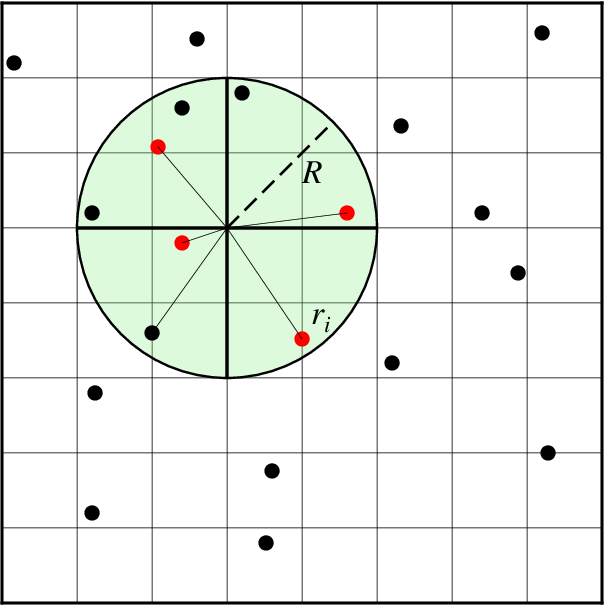
Search geometry for nearneighbor.
The GMT module nearneighbor implements a simple “nearest neighbor” averaging operation. It is the preferred way to grid data when the data density is high. nearneighbor is a local procedure which means it will only consider the control data that is close to the desired output grid node. Only data points inside a specified search radius will be used, and we may also impose the condition that each of the n sectors must have at least one data point in order to assign the nodal value. The nodal value is computed as a weighted average of the nearest data point per sector inside the search radius, with each point weighted according to its distance from the node. The most important switches are listed below.
Option |
Purpose |
|---|---|
-Sradius |
Sets search radius. Append unit for radius in that unit [Default is x-units] |
-Eempty |
Assign this value to unconstrained nodes [Default is NaN] |
-Nsectors |
Sector search, indicate number of sectors [Default is 4] |
-W |
Read relative weights from the 4th column of input data |
We will grid the data in the file tut_ship.xyz which contains ship observations of bathymetry off Baja California. We obtain the file via the cache server as before. We desire to make a 5’ by 5’ grid. Running gmt info on @tut_ship.xyz yields:
tut_ship.xyz: N = 82970 <245/254.705> <20/29.99131> <-7708/-9>
so we choose the region accordingly, and get a view of the contour map using
gmt begin GMT_tut_12
	gmt set GMT_THEME cookbook
	gmt nearneighbor -R245/255/20/30 -I5m -S40k -Gship.nc @tut_ship.xyz
	gmt grdcontour ship.nc -JM6i -B -C250 -A1000
gmt end show
Your plot should look like our example 12 below
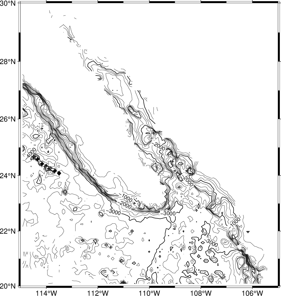
Result of GMT Tutorial example 12
Since the grid ship.nc is stored in netCDF format that is supported by a host of other modules, you can try one of those as well on the same grid.
Exercises:
Try using a 100 km search radius and a 10 minute grid spacing.
Gridding with Splines in Tension
As an alternative, we may use a global procedure to grid our data. This approach, implemented in the module surface, represents an improvement over standard minimum curvature algorithms by allowing users to introduce some tension into the surface. Physically, we are trying to force a thin elastic plate to go through all our data points; the values of this surface at the grid points become the gridded data. Mathematically, we want to find the function z(x, y) that satisfies the following equation away from data constraints:
where t is the “tension” in the 0-1 range. Basically, for zero tension we obtain the minimum curvature solution, while as tension goes toward unity we approach a harmonic solution (which is linear in cross-section). The theory behind all this is quite involved and we do not have the time to explain it all here, please see Smith and Wessel [1990] for details. Some of the most important switches for this module are indicated below.
Option |
Purpose |
|---|---|
-Aaspect |
Sets aspect ratio for anisotropic grids. |
-Climit |
Sets convergence limit. Default is 1/1000 of data range. |
-Ttension |
Sets the tension [Default is 0] |
Preprocessing
The surface module assumes that the data have been preprocessed to eliminate aliasing, hence we must ensure that this step is completed prior to gridding. GMT comes with three preprocessors, called blockmean, blockmedian, and blockmode. The first averages values inside the grid-spacing boxes, the second returns median values, wile the latter returns modal values. As a rule of thumb, we use means for most smooth data (such as potential fields) and medians (or modes) for rough, non-Gaussian data (such as topography). In addition to the required -R and -I switches, these preprocessors all take the same options shown below:
Option |
Purpose |
|---|---|
-r |
Choose pixel node registration [Default is gridline] |
-W[i|o] |
Append i or o to read or write weights in the 4th column |
With respect to our ship data we preprocess it using the median method:
gmt blockmedian -R245/255/20/30 -I5m -V @tut_ship.xyz > ship_5m.xyz
The output data can now be used with surface:
gmt surface ship_5m.xyz -R245/255/20/30 -I5m -Gship.nc -V
If you rerun grdcontour on the new grid file (try it!) you will notice a big difference compared to the grid made by nearneighbor: since surface is a global method it will evaluate the solution at all nodes, even if there are no data constraints. There are numerous options available to us at this point:
We can reset all nodes too far from a data constraint to the NaN value.
We can pour white paint over those regions where contours are unreliable.
We can plot the landmass which will cover most (but not all) of the unconstrained areas.
We can set up a clip path so that only the contours in the constrained region will show.
Here we have only time to explore the latter approach. The mask module can read the same preprocessed data and set up a contour mask based on the data distribution. Once the clip path is activated we can contour the final grid; we finally deactivate the clipping with a second call to mask. Here’s the recipe:
gmt blockmedian -R245/255/20/30 -I5m -V @tut_ship.xyz > ship_5m.xyz
gmt surface ship_5m.xyz -R245/255/20/30 -I5m -Gship.nc
gmt begin GMT_tut_13
	gmt set GMT_THEME cookbook
	gmt mask -R245/255/20/30 -I5m ship_5m.xyz -JM6i -B
	gmt grdcontour ship.nc -C250 -A1000
	gmt mask -C
gmt end show
Your plot should look like our example 13 below
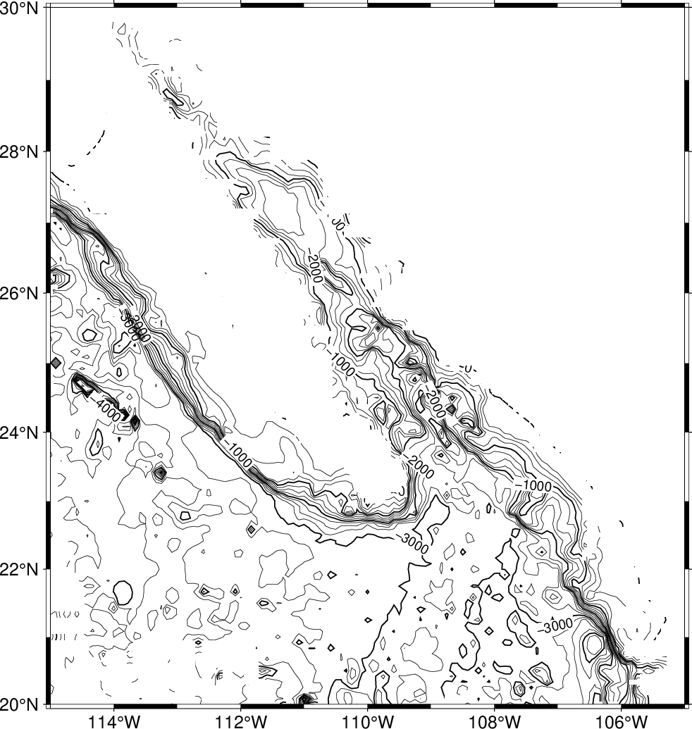
Result of GMT Tutorial example 13
Exercises:
Add the continents using any color you want.
Color the clip path light gray (use -G in the first mask call).