grdvector
Plot vector field from two component grids
Synopsis
gmt grdvector compx.nc compy.nc -Jparameters [ -A ] [ -B[p|s]parameters ] [ -Ccpt ] [ -Gfill ] [ -I[x]dx[/dy] ] [ -N ] [ -Qparameters ] [ -Rregion ] [ -S[i|l]scale ] [ -T ] [ -U[stamp] ] [ -Wpen ] [ -X[a|c|f|r][xshift] ] [ -Y[a|c|f|r][yshift] ] [ -Z ] [ -fflags ] [ -pflags ] [ -ttransp ] [ --PAR=value ]
Note: No space is allowed between the option flag and the associated arguments.
Description
grdvector reads two 2-D grid files which represents the x- and y-components of a vector field and produces a vector field plot by drawing vectors with orientation and length according to the information in the files. Alternatively, polar coordinate r, theta grids may be given instead.
Required Arguments
- compx.nc
Contains the x-components of the vector field. (See Grid File Formats).
- compy.nc
Contains the y-components of the vector field. (See Grid File Formats).
- -Jparameters
Specify the projection. (See full description) (See cookbook summary) (See projections table).
Optional Arguments
- -A
The grid files contain polar (r, theta) components instead of Cartesian (x, y) [Default is Cartesian components].
- -B[p|s]parameters
Set map boundary frame and axes attributes. (See full description) (See cookbook information).
- -C[cpt|master[+h[hinge]][+izinc][+u|Uunit] |color1,color2[,color3,…]]
Name of a CPT file. Alternatively, supply the name of a GMT color master dynamic CPT [turbo, but we use geo for @earth_relief and srtm for @srtm_relief data] to automatically determine a continuous CPT from the grid’s z-range; you may round the range to the nearest multiple of zinc by adding +izinc. If given a GMT Master soft-hinge CPT (see Of Colors and Color Legends) then you can enable the hinge at data value hinge [0] via +h, whereas for hard-hinge CPTs you can adjust the location of the hinge [0]. For other CPTs, you may convert their z-values from meter to another distance unit (append +Uunit) or from another unit to meter (append +uunit), with unit taken from e|f|k|M|n|u. Yet another option is to specify -Ccolor1,color2[,color3,…] to build a linear continuous CPT from those colors automatically. In this case colorn can be a r/g/b triplet, a color name, or an HTML hexadecimal color (e.g. #aabbcc). If no argument is given to -C then under modern mode we select the current CPT.
- -Gfill
Sets color or shade for vector interiors [Default is no fill].
- -I[x]dx[/dy]
Only plot vectors at nodes every x_inc, y_inc apart (must be multiples of original grid spacing). Append m for arc minutes or s for arc seconds. Alternatively, use -Ix to specify the multiples multx[/multy] directly [Default plots every node].
- -N
Do NOT clip vectors at map boundaries [Default will clip].
- -Qparameters
Modify vector parameters. For vector heads, append vector head size [Default is 0, i.e., stick-plot]. See VECTOR ATTRIBUTES for specifying additional attributes.
- -Rxmin/xmax/ymin/ymax[+r][+uunit]
Specify the region of interest. Specify a subset of the grid. (See full description) (See cookbook information).
- -S[i|l]scale
Sets scale for vector plot lengths in data units per plot distance measurement unit. Append c, i, or p to indicate the desired plot distance measurement unit (cm, inch, or point); if no unit is given we use the default value that is controlled by PROJ_LENGTH_UNIT. Vector lengths converted via plot unit scaling will plot as straight Cartesian vectors and their lengths are not affected by map projection and coordinate locations. For geographic data you may alternatively give scale in data units per map distance unit (see Units). Then, your vector magnitudes (in data units) are scaled to map distances in the given distance unit, and finally projected onto the Earth to give plot dimensions. These are geo-vectors that follow great circle paths and their lengths may be affected by the map projection and their coordinates. Finally, use -Si if it is simpler to give the reciprocal scale in plot length or distance units per data unit. To report the minimum, maximum, and mean data and plot vector lengths of all vectors plotted, use -V. Alternatively, use -Sllength to set a fixed plot length for all vectors.
- -T
Means the azimuths of Cartesian data sets should be adjusted according to the signs of the scales in the x- and y-directions [Leave alone]. This option can be used to convert vector azimuths in cases when a negative scale is used in one of both directions (e.g., positive down).
- -U[label|+c][+jjust][+odx/dy]
Draw GMT time stamp logo on plot. (See full description) (See cookbook information).
- -V[level]
Select verbosity level [w]. (See full description) (See cookbook information).
- -Wpen
Set pen attributes used for vector outlines [Default: width = default, color = black, style = solid].
- -X[a|c|f|r][xshift]
Shift plot origin. (See full description) (See cookbook information).
- -Y[a|c|f|r][yshift]
Shift plot origin. (See full description) (See cookbook information).
- -Z
The theta grid provided contains azimuths rather than directions (implies -A).
- -f[i|o]colinfo (more …)
Specify data types of input and/or output columns.
- -p[x|y|z]azim[/elev[/zlevel]][+wlon0/lat0[/z0]][+vx0/y0] (more …)
Select perspective view.
- -ttransp[/transp2] (more …)
Set transparency level(s) in percent.
- -^ or just -
Print a short message about the syntax of the command, then exit (NOTE: on Windows just use -).
- -+ or just +
Print an extensive usage (help) message, including the explanation of any module-specific option (but not the GMT common options), then exit.
- -? or no arguments
Print a complete usage (help) message, including the explanation of all options, then exit.
- --PAR=value
Temporarily override a GMT default setting; repeatable. See gmt.conf for parameters.
Units
For map distance unit, append unit d for arc degree, m for arc minute, and s for arc second, or e for meter [Default], f for foot, k for km, M for statute mile, n for nautical mile, and u for US survey foot. By default we compute such distances using a spherical approximation with great circles (-jg) using the authalic radius (see PROJ_MEAN_RADIUS). You can use -jf to perform “Flat Earth” calculations (quicker but less accurate) or -je to perform exact geodesic calculations (slower but more accurate; see PROJ_GEODESIC for method used).
Vector Attributes
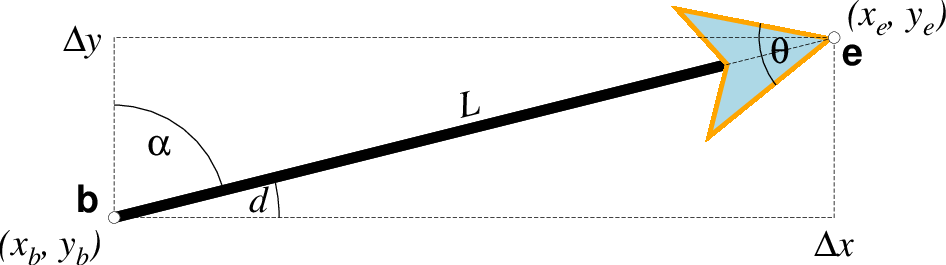
Vector attributes are controlled by options and modifiers. We will refer to this figure and the labels therein when introducing the corresponding modifiers. All vectors require you to specify the begin point \(x_b, y_b\) and the end point \(x_e, y_e\), or alternatively the direction d and length L, while for map projections we usually specify the azimuth \(\alpha\) instead.
Several modifiers may be appended to vector-producing options for specifying the placement of vector heads, their shapes, and the justification of the vector. Below, left and right refers to the side of the vector line when viewed from the beginning point (b) to the end point (e) of a line segment:
+aangle sets the angle \(\theta\) of the vector head apex [30].
+b places a vector head at the beginning of the vector path [none]. Optionally, append t for a terminal line, c for a circle, a for arrow [Default], i for tail, A for plain open arrow, and I for plain open tail. Further append l|r to only draw the left or right half-sides of this head [both sides].
+e places a vector head at the end of the vector path [none]. Optionally, append t for a terminal line, c for a circle, a for arrow [Default], i for tail, A for plain open arrow, and I for plain open tail. Further append l|r to only draw the left or right half-sides of this head [both sides].
+g[fill] sets the vector head fill [Default fill is used, which may be no fill]. Turn off vector head fill by not appending a fill. Some modules have a separate -Gfill option and if used will select the fill as well.
+hshape sets the shape of the vector head (range -2/2). Default is controlled by MAP_VECTOR_SHAPE [default is theme dependent]. A zero value produces no notch (e.g., the dashed line in the figure). Positive values moves the notch toward the head apex while a negative value moves away. The example above uses +h0.5.
+l draws half-arrows, using only the left side of specified heads [both sides].
+m places a vector head at the mid-point the vector path [none]. Append f or r for forward or reverse direction of the vector [forward]. Optionally, append t for a terminal line, c for a circle, a for arrow [Default], i for tail, A for plain open arrow, and I for plain open tail. Further append l|r to only draw the left or right half-sides of this head [both sides]. Cannot be combined with +b or +e.
+nnorm scales down vector attributes (pen thickness, head size) with decreasing length, where vector plot lengths shorter than norm will have their attributes scaled by length/norm [arrow attributes remains invariant to length]. For Cartesian vectors specify a length in plot units, while for geovectors specify a length in km.
+o[plon/plat] specifies the oblique pole for the great or small circles. Only needed for great circles if +q is given. If no pole is appended then we default to the north pole.
+p[pen] sets the vector pen attributes. If no pen is appended then the head outline is not drawn. [Default pen is half the width of stem pen, and head outline is drawn]. Above, we used +p2p,orange. The vector stem attributes are controlled by -W.
+q means the input direction, length data instead represent the start and stop opening angles of the arc segment relative to the given point. See +o to specify a specific pole for the arc [north pole].
+r draws half-arrows, using only the right side of specified heads [both sides].
+t[b|e]trim will shift the beginning or end point (or both) along the vector segment by the given trim; append suitable unit (c, i, or p). If the modifiers b|e are not used then trim may be two values separated by a slash, which is used to specify different trims for the beginning and end. Positive trims will shorted the vector while negative trims will lengthen it [no trim].
In addition, all but circular vectors may take these modifiers:
+jjust determines how the input x,y point relates to the vector. Choose from beginning [default], end, or center.
+s means the input angle, length are instead the \(x_e, y_e\) coordinates of the vector end point.
Finally, Cartesian vectors may take these modifiers:
+zscale expects input \(\Delta x, \Delta y\) vector components and uses the scale to convert to polar coordinates with length in given unit.
Note: Vectors were completely redesigned for GMT5 which separated the vector head (a polygon) from the vector stem (a line). In GMT4, the entire vector was a polygon and it could only be a straight Cartesian vector. Yes, the old GMT4 vector shape remains accessible if you specify a vector (-Sv|V) using the GMT4 syntax, explained here: size, if present, will be interpreted as \(t_w/h_l/h_w\) or tailwidth/headlength/halfheadwidth [Default is 0.075c/0.3c/0.25c (or 0.03i/0.12i/0.1i)]. By default, arrow attributes remain invariant to the length of the arrow. To have the size of the vector scale down with decreasing size, append +nnorm, where vectors shorter than norm will have their attributes scaled by length/norm. To center the vector on the balance point, use -Svb; to align point with the vector head, use -Svh; to align point with the vector tail, use -Svt [Default]. To give the head point’s coordinates instead of direction and length, use -Svs. Upper case B, H, T, S will draw a double-headed vector [Default is single head].
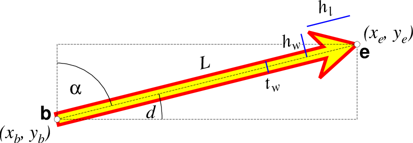
A GMT 4 vector has no separate pen for the stem -- it is all part of a Cartesian polygon. You may optionally fill and draw its outline. The modifiers listed above generally do not apply. Note: While the tailwidth (\(t_w\)) and headlength (\(h_l\)) parameters are given as indicated, the halfheadwidth (\(h_w\)) is oddly given as the half-width in GMT 4 so we retain that convention here (but have updated the documentation; blue lines indicate these three parameters).
Examples
Note: Below are some examples of valid syntax for this module.
The examples that use remote files (file names starting with @)
can be cut and pasted into your terminal for testing.
Other commands requiring input files are just dummy examples of the types
of uses that are common but cannot be run verbatim as written.
Note: Since many GMT plot examples are very short (i.e., one module call between the gmt begin and gmt end commands), we will often present them using the quick modern mode GMT Modern Mode One-line Commands syntax, which simplifies such short scripts.
To draw the vector field given by the files r.nc and theta.nc on a linear plot with scale 5 cm per data unit, using vector rather than stick plot, scale vector magnitudes so that 10 units equal 1 inch, and center vectors on the node locations, run
gmt grdvector r.nc theta.nc -Jx5c -A -Q0.1i+e+jc -S10i -pdf gradient
To plot a geographic data sets given the files comp_x.nc and comp_y.nc, using a length scale of 200 km per data unit and only plot every 3rd node in either direction, try
gmt grdvector comp_x.nc comp_y.nc -Ix3 -JH0/20c -Q0.1i+e+jc -S200k -pdf globe
Vector scaling and unit effects
The scale given via -S may require some consideration. As explained in -S, it is specified in data-units per plot or distance unit. The plot or distance unit chosen will affect the type of vector you select. In all cases, we first compute the magnitude r of the user’s data vectors at each selected node from the x and y components (unless you are passing r, theta grids directly with -A). These magnitudes are given in whatever data units they come with. Let us pretend our data grids record secular changes in the Earth’s magnetic horizontal vector field in units of nTesla/year, and that at a particular node the magnitude is 28 nTesla/year (in some direction). If you specify the scale using plot distance units (c|i|p) then you are selecting Cartesian vectors. Let us further pretend that you selected -S10c as your scale option. That means you want 10 nTesla/year to equate to a 1 cm plot length. Internally, we convert this scale to a plot scale of 1/10 = 0.1 cm per nTesla/year. Given our vector magnitude of 28 nTesla/year, we multiply it by our plot scale and finally obtain a vector length of 2.8 cm, which is then plotted. The user’s data units do not enter of course, i.e., they always cancel [Likewise, if we had used -S25i (25 nTesla/year per inch) the plot scale would be (1/25) = 0.04 inch per nTesla/year and the vector plot lengths would be 28 * 0.04 inch = 1.12 inch]. If we now wished to plot a 10 nTesla/year reference vector in the map legend we would plot one that is 10 times 0.1 cm = 1 cm long since the scale length is constant regardless of map projection and location. A 10 nTesla/year vector will be 1 cm anywhere.
Let us contrast this behavior with what happens if we use a geographic distance unit instead, say -S0.5k (0.5 nTesla/year per km). Internally, this becomes a map scale of 2 km per nTesta/year. Given our node magnitude of 28 nTesla/year, the vector length will be 28 x 2 km = 56 km. Again, the user’s data unit do not enter. Now, that vector length of 56 km must be projected onto the Earth, and because of map distortions, a 56 km vector will be mapped to a length on the plot that is a function of the user’s map projection, the map scale, and possibly the location on the map. E.g., a 56 km vector due east at Equator on a Mercator map would seem to equal ~0.5 degree longitude but at 60 north it would be more like ~1 degree longitude. A consequence of this effect is that a user who wants to add a 10 nTesla/year reference vector to a legend faces the same problem we do when we wish to draw a 100 km map scale on a map: the plotted length usually will depend on latitude and hence that reference scale is only useful around that latitude.
This brings us to the inverse scale option, -Silength. This variant is useful when providing the inverse of the scale is simpler. In the Cartesian case above, we could instead give -Si0.1c which would directly imply a plot scale of 0.1 cm per nTesla/year. Likewise, for geographic distances we could give -Si2k for 2 km per nTesla/year scale as well. As the -Si argument increases, the plotted vector length increases as well, while for plain -S the plot length decreases with increasing scale.
Notes
Be aware that using -I may lead to aliasing unless your grid is smoothly varying over the new length increments. It is generally better to filter your grids and resample at a larger grid increment and use these grids instead of the originals.