Session One
Tutorial setup
We assume that GMT has been properly and fully installed and that the GMT executables are in your executable path. You should be able to type
gmtin your terminal and it will display the GMT splash screen with version number and the top-level options. If not then you need to work on your user environment, adding the path to the gmt executable to your search path.All GMT man pages, documentation, and gallery example scripts are available from the GMT documentation web page. It is assumed these pages have been installed locally at your site; if not they are always available from https://docs.generic-mapping-tools.org.
We recommend you create a sub-directory called tutorial, cd into that directory, and run the commands there to keep things tidy.
As we discuss GMT principles it may be a good idea to consult the GMT Cookbook for more detailed explanations.
The tutorial data sets are distributed via the GMT cache server. You will therefore find that all the data files have a “@” prepended to their names. This will ensure the file is copied from the server before being used, hence you do not need to download any of the data manually. The only downside is that you will need an Internet connection to run the examples by cut and paste.
For all but the simplest GMT jobs it is recommended that you place all the GMT (and UNIX) commands in a shell script file and make it executable. To ensure that UNIX recognizes your script as a shell script it is a good habit always to start the script with the line
#!/usr/bin/env bashor#!/usr/bin/env csh, depending on the shell you prefer to use. All the examples in this tutorial assumes you are running the Bourne Again shell, bash, and you will need to modify some of the constructs, such as i/o redirection, to run these examples under csh. We strongly recommend bash over csh due the ability to define functions.Making a script executable is accomplished using the chmod command, e.g., the script figure_1.sh is made executable with “chmod +x figure_1.sh”.
Please cd into the directory tutorial. We are now ready to start.
The GMT environment: What happens when you run GMT ?
To get a good grasp on GMT one must understand what is going on “under the hood”. The GMT Run-Time Environment illustrates the relationships you need to be aware of at run-time.
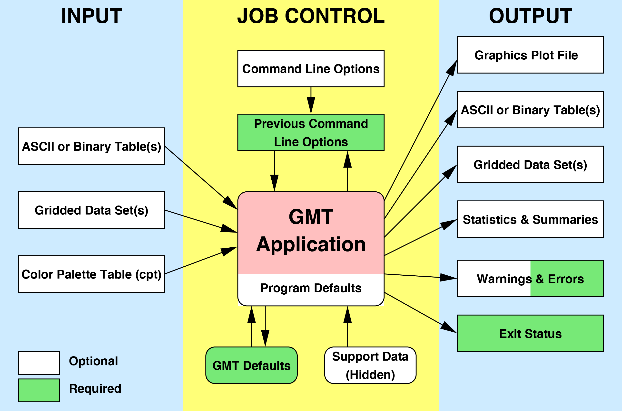
The GMT run-time environment. The will initiate with a set of system defaults that you can override with having your own gmt.conf file in the current directory, specifying GMT parameters via the --PAR=value technique, and supply module options. Some GMT modules will read hidden data (like coastlines) but most will explicitly need to be given user data.
Input data
A GMT module may or may not take input files. Three different types of input are recognized (more details can be found in GMT File Formats):
Data tables. These are rectangular tables with a fixed number of columns and unlimited number of rows. We distinguish between two groups:
ASCII (Preferred unless files are huge)
Binary (to speed up input/output)
Such tables may have segment headers and can therefore hold any number of subsets such as individual line segments or polygons.
Gridded dated sets. These are data matrices (evenly spaced in two coordinates) that come in two flavors:
Grid-line registration
Pixel registration
You may choose among several file formats (even define your own format), but the GMT default is the architecture-independent netCDF format.
Color palette table (For imaging, color plots, and contour maps). We will discuss these later.
Job Control
GMT modules may get operational parameters from several places:
Supplied command line options/switches or module defaults.
Short-hand notation to select previously used option arguments (stored in gmt.history).
Implicitly using GMT defaults for a variety of parameters (stored in gmt.conf).
May use hidden support data like coastlines or PostScript patterns.
Output data
There are 6 general categories of output produced by GMT:
PostScript plot commands.
Data Table(s).
Gridded data set(s).
Statistics & Summaries.
Warnings and Errors, written to stderr.
Exit status (0 means success, otherwise failure).
Note: GMT automatically creates and updates a history of past GMT command options for the common switches. This history file is called gmt.history and one will be created in every directory from which GMT modules are executed. Many initial problems with GMT usage result from not fully appreciating the relationships shown in Figure GMT Environment .
The UNIX Environment: Entry Level Knowledge
Redirection
Most GMT modules read their input from the terminal (called stdin) or from files, and write their output to the terminal (called stdout). To use files instead one can use redirection:
gmt module input-file > output-file         # Read a file and redirect output
gmt module < input-file > output-file       # Redirect input and output
gmt module input-file >> output-file        # Append output to existing file
In this example, and in all those to follow, it is assumed that you do not have the shell variable noclobber set. If you do, it prevents accidental overwriting of existing files. That may be a noble cause, but it is extremely annoying. So please, unset noclobber.
Piping (|)
Sometimes we want to use the output from one module as input to another module. This is achieved with pipes:
Someprogram | gmt module1 | gmt module1 > OutputFile
Standard error (stderr)
Most programs and GMT modules will on occasion write error messages. These are typically written to a separate data stream called stderr and can be redirected separately from the standard output (which goes to stdout). To send the error messages to the same location as standard output we use:
program > errors.log 2>&1
When we want to save both program output and error messages to separate files we use the following syntax:
gmt module > output.txt 2> errors.log
File name expansion or “wild cards”
UNIX provides several ways to select groups of files based on name patterns:
Code |
Meaning |
|---|---|
* |
Matches anything |
? |
Matches any single character |
list |
Matches characters in the list |
range |
Matches characters in the given range |
You can save much time by getting into the habit of selecting “good” filenames that make it easy to select subsets of all files using the UNIX wild card notation.
Examples:
gmt module data_*.txt operates on all files starting with “data_” and ending in “.txt”.
gmt module line_?.txt works on all files starting with “line_” followed by any single character and ending in “.txt”.
gmt module section_1[0-9]0.part_[12] only processes data from sections 100 through 190, only using every 10th profile, and gets both part 1 and 2.
Laboratory Exercises
We will begin our adventure by making some simple plot axes and coastline basemaps. We will do this in order to introduce the all-important common options -B, -J, and -R and to familiarize ourselves with a few selected GMT projections. The GMT modules we will utilize are basemap and coast. Please consult their manual pages for reference.
Linear projection
We start by making the basemap frame for a linear x-y plot. We want it to go from 10 to 70 in x and from -3 to 8 in y, with automatic annotation intervals. Finally, we let the canvas be painted light red and have dimensions of 4 by 3 inches. Here’s how we do it:
gmt begin GMT_tut_1
	gmt basemap -R10/70/-3/8 -JX4i/3i -B -B+glightred+t"My first plot"
gmt end show
This script will open the result GMT_tut_1.pdf in a PDF viewer and it should look like our example 1 below. Examine the basemap documentation so you understand what each option means.
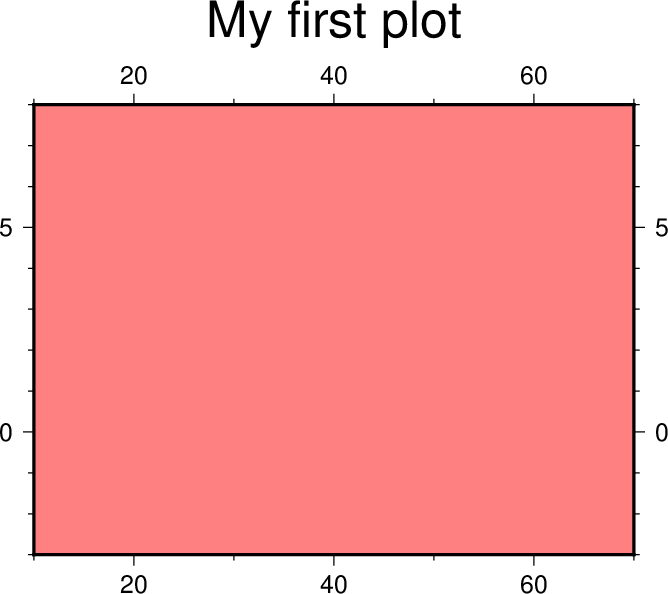
Result of GMT Tutorial example 1.
Exercises:
Try change the -JX values.
Try change the -B values.
Change title and canvas color.
Logarithmic projection
We next will show how to do a basemap for a log–log plot. We have no data set yet but we will imagine that the raw x data range from 3 to 9613 and that y ranges from 10^20 to 10^24. One possibility is
gmt begin GMT_tut_2
	gmt basemap -R1/10000/1e20/1e25 -JX9il/6il -Bxa2+l"Wavelength (m)" -Bya1pf3+l"Power (W)" -BWS
gmt end show
Make sure your plot looks like our example 2 below
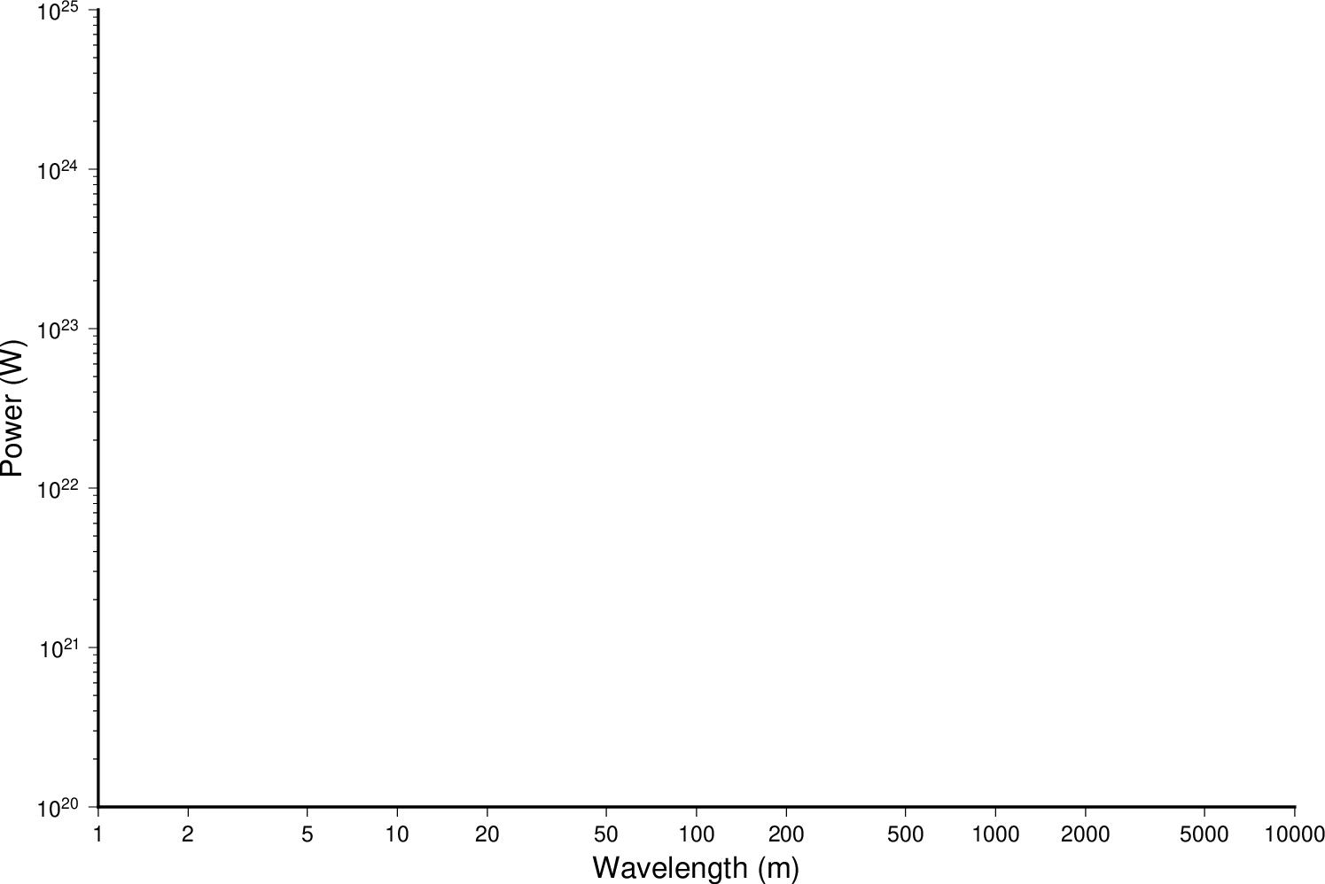
Result of GMT Tutorial example 2.
Exercises:
Do not append l to the axes lengths.
Leave the p modifier out of the -B string.
Add g3 to -Bx and -By.
Mercator projection
Despite the problems of extreme horizontal exaggeration at high latitudes, the conformal Mercator projection (-JM) remains the stalwart of location maps used by scientists. It is one of several cylindrical projections offered by GMT; here we will only have time to focus on one such projection. The complete syntax is simply
-JMwidth
To make coastline maps we use coast which automatically will access the GMT coastline, river and border data base derived from the GSHHG database [See Wessel and Smith, 1996]. In addition to the common switches we may need to use some of several coast-specific options:
Option |
Purpose |
|---|---|
-A |
Exclude small features or those of high hierarchical levels (see GSHHG) |
-D |
Select data resolution (full, high, intermediate, low, or crude) |
-G |
Set color of dry areas (default does not paint) |
-I |
Draw rivers (chose features from one or more hierarchical categories) |
-L |
Plot map scale (length scale can be km, miles, or nautical miles) |
-N |
Draw political borders (including US state borders) |
-S |
Set color for wet areas (default does not paint) |
-W |
Draw coastlines and set pen thickness |
One of -W, -G, -S must be selected. Our first coastline example is from Latin America:
gmt begin GMT_tut_3
	gmt coast -R-90/-70/0/20 -JM6i -B -Gchocolate
gmt end show
Your plot should look like our example 3 below
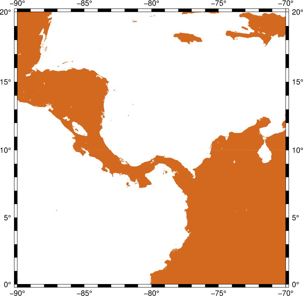
Result of GMT Tutorial example 3.
Exercises:
Add the -V option.
Try -R270/290/0/20 instead. What happens to the annotations?
Edit your gmt.conf file, change FORMAT_GEO_MAP to another setting (see the gmt.conf documentation), and plot again.
Pick another region and change land color.
Pick a region that includes the north or south poles.
Try -W0.25p instead of (or in addition to) -G.
Albers projection
The Albers projection (-JB) is an equal-area conical projection; its conformal cousin is the Lambert conic projection (-JL). Their usages are almost identical so we will only use the Albers here. The general syntax is
-JBlon_0/lat_0/lat_1/lat_2/width
where (lon_0, lat_0) is the map (projection) center and lat_1, lat_2 are the two standard parallels where the cone intersects the Earth’s surface. We try the following command:
gmt begin GMT_tut_4
	gmt coast -R-130/-70/24/52 -JB-100/35/33/45/6i -B -B+t"Conic Projection" -N1/thickest -N2/thinnest -A500 -Ggray -Wthinnest
gmt end show
Your plot should look like our example 4 below
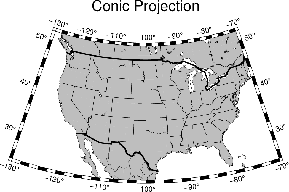
Result of GMT Tutorial example 4.
Exercises:
Change the parameter MAP_GRID_CROSS_SIZE_PRIMARY to make grid crosses instead of gridlines.
Change -R to a rectangular box specification instead of minimum and maximum values.
Orthographic projection
The azimuthal orthographic projection (-JG) is one of several projections with similar syntax and behavior; the one we have chosen mimics viewing the Earth from space at an infinite distance; it is neither conformal nor equal-area. The syntax for this projection is
-JGlon_0/lat_0/width
where (lon_0, lat_0) is the center of the map (projection). As an example we will try
gmt begin GMT_tut_5
	gmt coast -Rg -JG280/30/6i -Bag -Dc -A5000 -Gwhite -SDarkTurquoise
gmt end show
Your plot should look like our example 5 below

Result of GMT Tutorial example 5
Exercises:
Use the rectangular option in -R to make a rectangular map showing the US only.
Eckert IV and VI projection
We conclude the survey of map projections with the Eckert IV and VI projections (-JK), two of several projections used for global thematic maps; They are both equal-area projections whose syntax is
-JK[f|s]lon_0/width
where b gives Eckert IV (4) and s (Default) gives Eckert VI (6). The lon_0 is the central meridian (which takes precedence over the mid-value implied by the -R setting). A simple Eckert VI world map is thus generated by
gmt begin GMT_tut_6
	gmt coast -Rg -JKs180/9i -Bag -Dc -A5000 -Gchocolate -SDarkTurquoise -Wthinnest
gmt end show
Your plot should look like our example 6 below
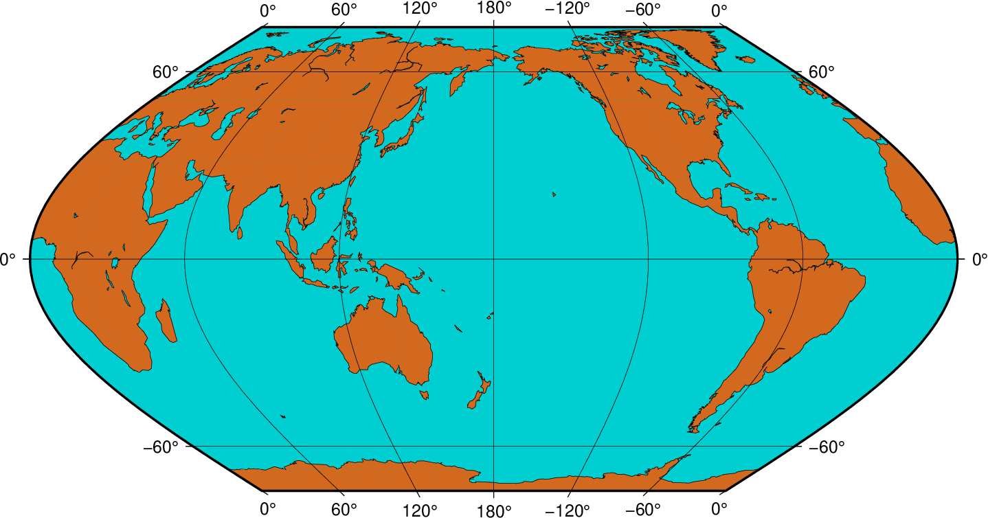
Result of GMT Tutorial example 6
Exercises:
Center the map on Greenwich.
Add a map scale with -L.