Session Four
In our final session we will concentrate on color images and perspective views of gridded data sets. Before we start that discussion we need to cover three important aspects of plotting that must be understood. These are
- Color tables and pseudo-colors in GMT.
- Artificial illumination and how it affects colors.
- Multi-dimensional grids.
CPTs
The CPT is discussed in detail in the GMT Technical Reference and Cookbook. Please review the format before experimenting further.
CPTs can be created in any number of ways. GMT provides two mechanisms:
- Create simple, linear color tables given a master color table (several are built-in) and the desired z-values at color boundaries (makecpt)
- Create color tables based on a master CPT color table and the histogram-equalized distribution of z-values in a gridded data file (grd2cpt)
One can also make these files manually or with awk or other tools. Here we will limit our discussion to makecpt. Its main argument is the name of the master color table (a list is shown if you run the module with no arguments) and the equidistant z-values to go with it. The main options are given below.
Option Purpose -C Set the name of the master CPT to use -I Reverse the sense of the color progression -V Run in verbose mode -Z Make a continuous rather than discrete table
To make discrete and continuous color CPTs for data that ranges from -20 to 60, with color changes at every 10, try these two variants:
gmt makecpt -Crainbow -T-20/60/10 > disc.cpt
gmt makecpt -Crainbow -T-20/60/10 -Z > cont.cpt
We can plot these color tables with colorbar; the options worth mentioning here are listed below. The placement of the color bar is particularly important and we refer you to the Plot embellishments section for all the details. In addition, the -B option can be used to set the title and unit label (and optionally to set the annotation-, tick-, and grid-line intervals for the color bars.). Note that the makecpt commands above are done in classic mode. If you run makecpt in modern mode then you usually do not specify an output file via stdout since modern mode maintains what is known as the current CPT. However, if you must explicitly name an output CPT then you will need to add the -H option for modern mode to allow output to stdout.
Option Purpose -Ccpt The required CPT -Dxxpos/ypos+wlength/width[+h] Sets the position and dimensions of scale bar. Append +h to get horizontal bar -Imax_intensity Add illumination effects
Here is an example of four different ways of presenting the color bar:
gmt begin GMT_tut_14
	gmt makecpt -H -Crainbow -T-20/60/10 > disc.cpt
	gmt makecpt -H -Crainbow -T-20/60 > cont.cpt
	gmt basemap -R0/6/0/9 -Jx1i -B0 -Xc
	gmt colorbar -Dx1i/1i+w4i/0.5i+h -Cdisc.cpt -Ba -B+tdiscrete
	gmt colorbar -Dx1i/3i+w4i/0.5i+h -Ccont.cpt -Ba -B+tcontinuous
	gmt colorbar -Dx1i/5i+w4i/0.5i+h -Cdisc.cpt -Ba -B+tdiscrete -I0.5
	gmt colorbar -Dx1i/7i+w4i/0.5i+h -Ccont.cpt -Ba -B+tcontinuous -I0.5
gmt end show
Your plot should look like our example 14 below
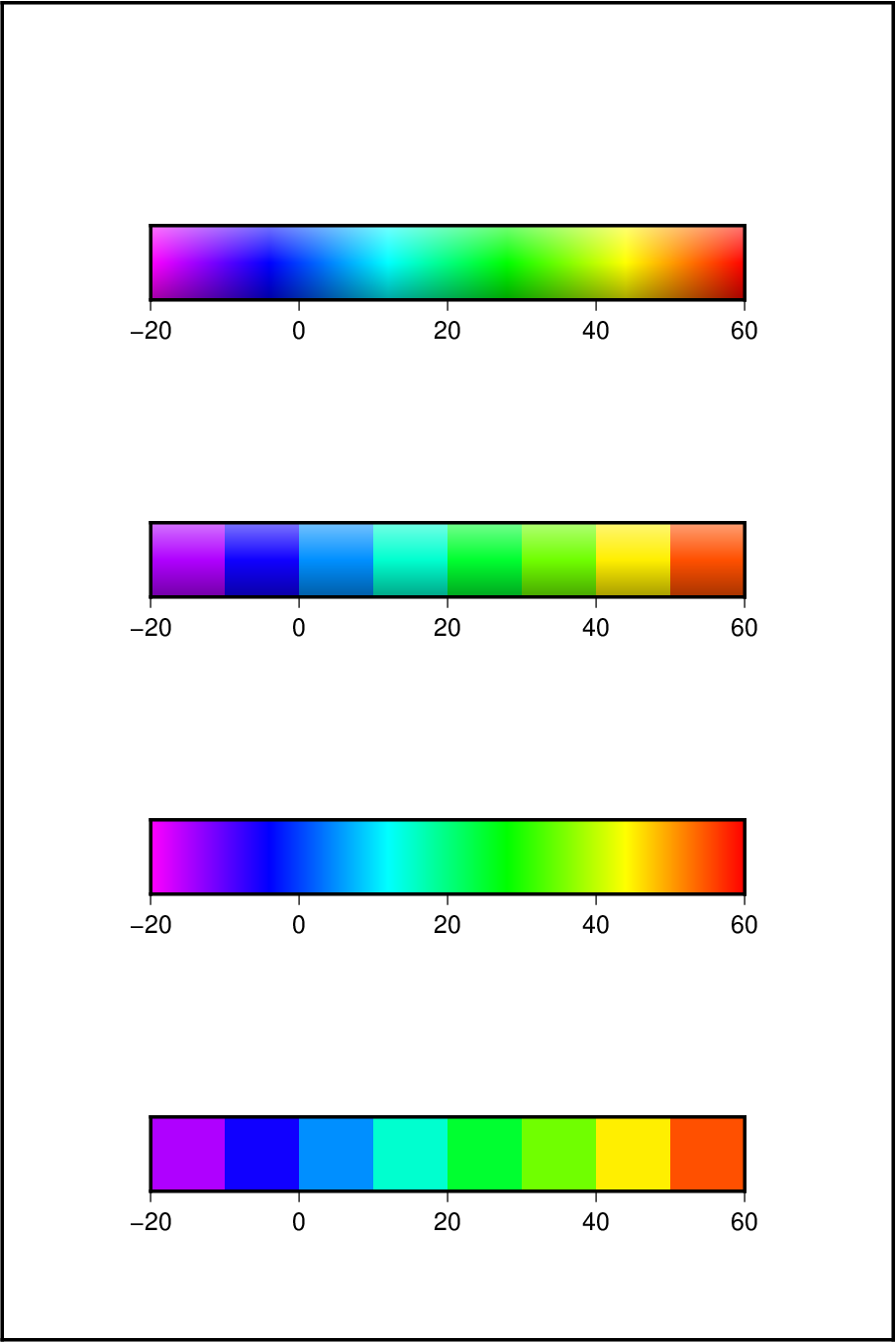
Result of GMT Tutorial example 14
Exercises:
- Redo the makecpt exercise using the master table hot and redo the bar plot.
- Try specifying -B10g5.
Illumination and intensities
GMT allows for artificial illumination and shading. What this means is that we imagine an artificial sun placed at infinity in some azimuth and elevation position illuminating our surface. The parts of the surface that slope toward the sun should brighten while those sides facing away should become darker; no shadows are cast as a result of topographic undulations.
While it is clear that the actual slopes of the surface and the orientation of the sun enter into these calculations, there is clearly an arbitrary element when the surface is not topographic relief but some other quantity. For instance, what does the slope toward the sun mean if we are plotting a grid of heat flow anomalies? While there are many ways to accomplish what we want, GMT offers a relatively simple way: We may calculate the gradient of the surface in the direction of the sun and normalize these values to fall in the -1 to +1 range; +1 means maximum sun exposure and -1 means complete shade. Although we will not show it here, it should be added that GMT treats the intensities as a separate data set. Thus, while these values are often derived from the relief surface we want to image they could be separately observed quantities such as back-scatter information.
Colors in GMT are specified in the RGB system used for computer screens; it mixes red, green, and blue light to achieve other colors. The RGB system is a Cartesian coordinate system and produces a color cube. For reasons better explained in Appendix I in the Reference book it is difficult to darken and brighten a color based on its RGB values and an alternative coordinate system is used instead; here we use the HSV system. If you hold the color cube so that the black and white corners are along a vertical axis, then the other 6 corners project onto the horizontal plane to form a hexagon; the corners of this hexagon are the primary colors Red, Yellow, Green, Cyan, Blue, and Magenta. The CMY colors are the complimentary colors and are used when paints are mixed to produce a new color (this is how printers operate; they also add pure black (K) to avoid making gray from CMY). In this coordinate system the angle 0-360º is the hue (H); the Saturation and Value are harder to explain. Suffice it to say here that we intend to darken any pure color (on the cube facets) by keeping H fixed and adding black and brighten it by adding white; for interior points in the cube we will add or remove gray. This operation is efficiently done in the HSV coordinate system; hence all GMT shading operations involve translating from RGB to HSV, do the illumination effect, and transform back the modified RGB values.
Color images
Once a CPT has been made it is relatively straightforward to generate a color image of a gridded data. Here, we will extract a subset of the global 30” DEM called SRTM30+:
gmt grdcut @earth_relief_30s -R-108/-103/35/40 -Gtut_relief.nc
Using grdinfo we find that the data ranges from about 1000m to about 4300m so we need to make a CPT with that range.
Color images are made with grdimage which takes the usual common command options (by default the -R is taken from the data set) and a CPT; the main other options are:
Option Purpose -Edpi Sets the desired resolution of the image [Default is data resolution] -Iintenfile Use artificial illumination using intensities from intensfile -M Force gray shade using the (television) YIQ conversion
We want to make a plain color map with a color bar superimposed above the plot. We try
gmt begin GMT_tut_15
	gmt makecpt -Crainbow -T1000/5000
	gmt grdimage @tut_relief.nc -JM6i -B -BWSnE
	gmt colorbar -DJTC -I0.4 -Bxa -By+lm
gmt end show
Your plot should look like our example 15 below
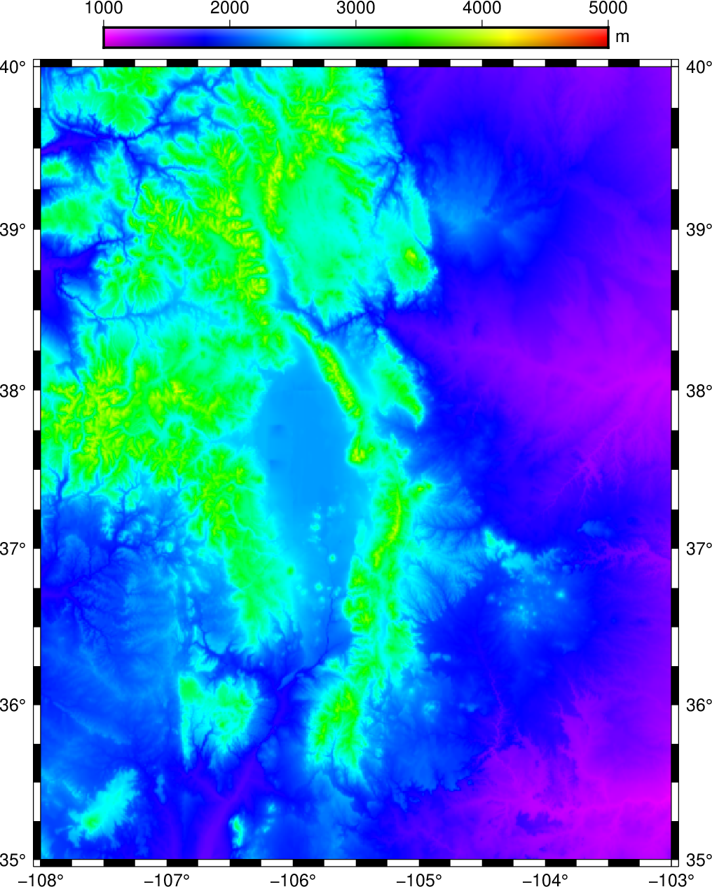
Result of GMT Tutorial example 15
The plain color map lacks detail and fails to reveal the topographic complexity of this Rocky Mountain region. What it needs is artificial illumination. We want to simulate shading by a sun source in the east, hence we derive the required intensities from the gradients of the topography in the N90ºE direction using grdgradient. Other than the required input and output filenames, the available options are
Option Purpose -Aazimuth Azimuthal direction for gradients -fg Indicates that this is a geographic grid -N[t|e][+snorm][+ooffset] Normalize gradients by norm/offset [= 1/0 by default]. Insert t to normalize by the inverse tangent transformation. Insert e to normalize by the cumulative Laplace distribution.
The GMT inverse tangent transformation shows that raw slopes from bathymetry tend to be far from normally distributed (left). By using the inverse tangent transformation we can ensure a more uniform distribution (right). The inverse tangent transform simply takes the raw slope estimate (the x value at the arrow) and returns the corresponding inverse tangent value (normalized to fall in the plus/minus 1 range; horizontal arrow pointing to the y-value).
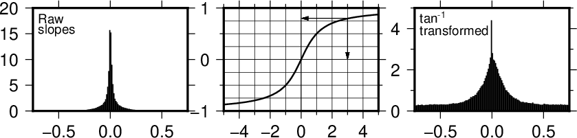
How the inverse tangent operation works. Raw slope values (left) are processed via the inverse tangent operator, turning tan(x) into x and thus compressing the data range. The transformed slopes are more normally distributed (right).
-Ne and -Nt yield well behaved gradients. Personally, we prefer to use the -Ne option; the value of norm is subjective and you may experiment somewhat in the 0.5-5 range. For our case we choose
gmt grdgradient @tut_relief.nc -Ne0.8 -A100 -fg -Gus_i.nc
Given the CPT and the two gridded data sets we can create the shaded relief image:
gmt begin GMT_tut_16
	gmt makecpt -Crainbow -T1000/5000
	gmt grdgradient @tut_relief.nc -Ne0.8 -A100 -fg -Gus_i.nc
	gmt grdimage tut_relief.nc -Ius_i.nc -JM6i -B -BWSnE
	gmt colorbar -DJTC -I0.4 -Bxa -By+lm
gmt end show
Your plot should look like our example 16 below
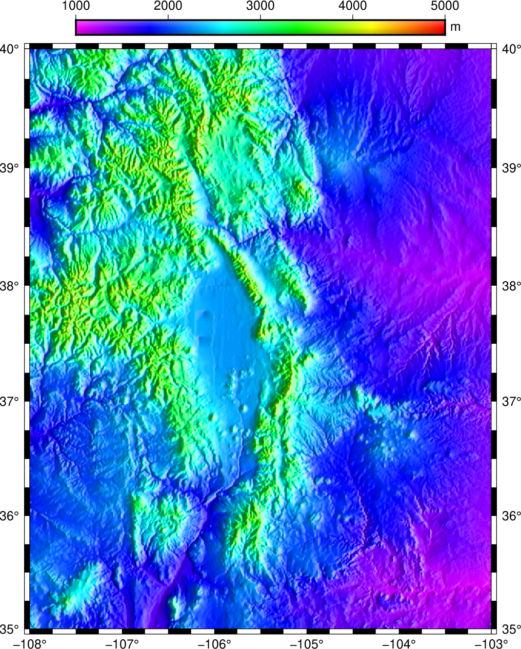
Result of GMT Tutorial example 16
Exercises:
- Force a gray-shade image.
- Rerun grdgradient with -N1.
Multi-dimensional maps
Climate data, like ocean temperatures or atmospheric pressure, are often provided as multi-dimensional (3-D, 4-D or 5-D) grids in netCDF format. This section will demonstrate that GMT is able to plot “horizontal” slices (spanning latitude and longitude) of such grids without much effort.
As an example we will download the Seasonal Analysed Mean Temperature from the World Ocean Atlas 1998 The file in question is named otemp.anal1deg.nc (ftp://ftp.cdc.noaa.gov/Datasets/nodc.woa98/temperat/seasonal/otemp.anal1deg.nc).
You can look at the information pertained in this file using the program ncdump and notice that the variable that we want to plot (otemp) is a four-dimensional variable of time, level (i.e., depth), latitude and longitude.
ncdump -h otemp.anal1deg.nc
We will need to make an appropriate color scale, running from -2ºC (freezing temperature of salt water) to 30ºC (highest likely ocean temperature). Let us focus on the temperatures in Summer (that is the third season, July through September) at sea level (that is the first level). To plot these in a Mollweide projection we use:
gmt begin GMT_tut_17
	gmt makecpt -Cno_green -T-2/30/2
	gmt grdimage -Rg -JW180/9i "@otemp.anal1deg.nc?otemp[2,0]" -Bag
gmt end show
The addition “?otemp[2,0]” indicates which variable to retrieve from the netCDF file (otemp) and that we need the third time step and first level. The numbering of the time steps and levels starts at zero, therefore “[2,0]”. Make sure to put the whole file name within quotes since the characters ?, [ and ] have special meaning in Unix. Your plot should look like our example 17 below
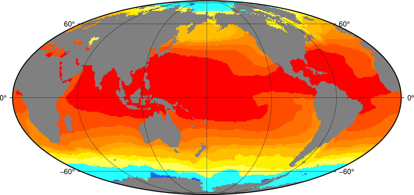
Result of GMT Tutorial example 17
Exercises:
- Plot the temperatures for Spring at 5000 m depth. (Hint: use ncdump -v level to figure out what level number that is).
- Include a color scale at the bottom of the plot.
Perspective views
Our final undertaking in this tutorial is to examine three-dimensional perspective views. The GMT module that produces perspective views of gridded data files is grdview. It can make two kinds of plots:
- Mesh or wire-frame plot (with or without superimposed contours)
- Color-coded surface (with optional shading, contours, or draping).
Regardless of plot type, some arguments must be specified; these are
- relief_file; a gridded data set of the surface.
- -J for the desired map projection.
- -JZheight for the vertical scaling.
- -pazimuth/elevation for the vantage point.
In addition, some options may be required:
Option Purpose -Ccpt The cpt is required for color-coded surfaces and for contoured mesh plots -Gdrape_file Assign colors using drape_file instead of relief_file -Iintens_file File with illumination intensities -Qm Selects mesh plot -Qs[+m] Surface plot using polygons; append +m to show mesh. This option allows for -W -Qidpi[g] Image by scan-line conversion. Specify dpi; append g to force gray-shade image. -B is disabled. -Wpen Draw contours on top of surface (except with -Qi)
Mesh-plot
Mesh plots work best on smaller data sets. We again use the small subset of the ETOPO5 data over Bermuda and will use the ocean CPT. A simple mesh plot can therefore be obtained with
gmt begin GMT_tut_18
	gmt grd2cpt @tut_bathy.nc -Cocean
	gmt grdview tut_bathy.nc -JM5i -JZ2i -p135/30 -B
gmt end show
Your plot should look like our example 18 below
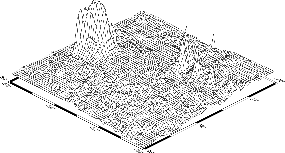
Result of GMT Tutorial example 18
Exercises:
- Select another vantage point and vertical height.
Color-coded view
We will make a perspective, color-coded view of the US Rockies from the southeast. This is done using
gmt begin GMT_tut_19
	gmt makecpt -Ctopo -T1000/5000
	gmt grdgradient @tut_relief.nc -Ne0.8 -A100 -fg -Gus_i.nc
	gmt grdview tut_relief.nc -JM4i -p135/35 -Qi50 -Ius_i.nc -B -JZ0.5i -C
gmt end show
Your plot should look like our example 19 below
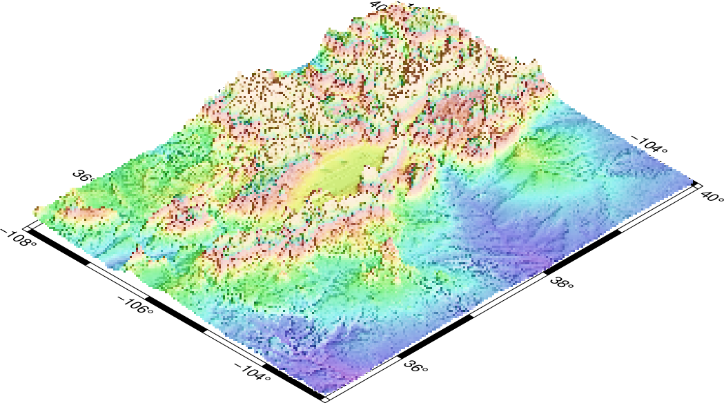
Result of GMT Tutorial example 19
This plot is pretty crude since we selected 50 dpi but it is fast to render and allows us to try alternate values for vantage point and scaling. When we settle on the final values we select the appropriate dpi for the final output device and let it rip.
Exercises:
- Choose another vantage point and scaling.
- Redo grdgradient with another illumination direction and plot again.
- Select a higher dpi, e.g., 200.