Session One
Tutorial setup
GMT man pages, documentation, and gallery example scripts are available from the GMT.jl documentation web page available from https://www.generic-mapping-tools.org/GMT.jl/dev/.
We recommend you create a sub-directory called tutorial, cd into that directory, and run the commands there to keep things tidy.
As we discuss GMT principles it may be a good idea to consult the GMT Cookbook for more detailed explanations (but the CookBook is not translated into the GMT.jl syntax).
The tutorial data sets are distributed via the GMT cache server. You will therefore find that all the data files have a “@” prepended to their names. This will ensure the file is copied from the server before being used, hence you do not need to download any of the data manually. The only downside is that you will need an Internet connection to run the examples by cut and paste.
Please cd into the directory tutorial. We are now ready to start.
Input data
A GMT module may or may not take input data/files. Four different types of input are recognized (more details can be found in GMT File Formats):
Data tables. These are rectangular tables with a fixed number of columns and unlimited number of rows. We distinguish between two groups:
ASCII (Preferred unless files are huge)
Binary (to speed up input/output)
In memory GMTdataset or plain Julia matrices.
Such tables may have segment headers and can therefore hold any number of subsets such as individual line segments or polygons.
Gridded dated sets. These are data matrices (evenly spaced in two coordinates) that come in two flavors:
Grid-line registration
Pixel registration
You may choose among several file formats (even define your own format), but the GMT default is the architecture-independent netCDF format.
The other alternative is to use Julia in-memory data in the form of GMTgrids.
Color palette table (For imaging, color plots, and contour maps). We will discuss these later.
Job Control
GMT modules may get operational parameters from several places:
Supplied command line options/switches or module defaults.
Short-hand notation to select previously used option arguments.
Implicitly using GMT defaults for a variety of parameters (stored in gmt.conf).
May use hidden support data like coastlines or PostScript patterns.
Output data
There are 5 general categories of output produced by GMT:
PostScript plot commands.
Data Table(s).
Gridded data set(s).
Statistics & Summaries.
Warnings and Errors, written to the REPL
Laboratory Exercises
We will begin our adventure by making some simple plot axes and coastline basemaps. We will do this in order to introduce the all-important common options frame, proj, and region and to familiarize ourselves with a few selected GMT projections. The GMT modules we will utilize are basemap and basemap. Please consult their manual pages for reference.
Linear projection
We start by making the basemap frame for a linear x-y plot. We want it to go from 10 to 70 in x and from -3 to 8 in y, with automatic annotation intervals. Finally, we let the canvas be painted light red and have dimensions of 10 by 7.5 centimeters. Here’s how we do it:
basemap(region=(10,70,-3,8), proj=:linear, figsize=(10,7.5),
        frame=(fill=:lightred, title="My first plot"), show=true)
This script will open the result in a PNG viewer and it should look like our example 1 below. Examine the basemap documentation so you understand what each option means.
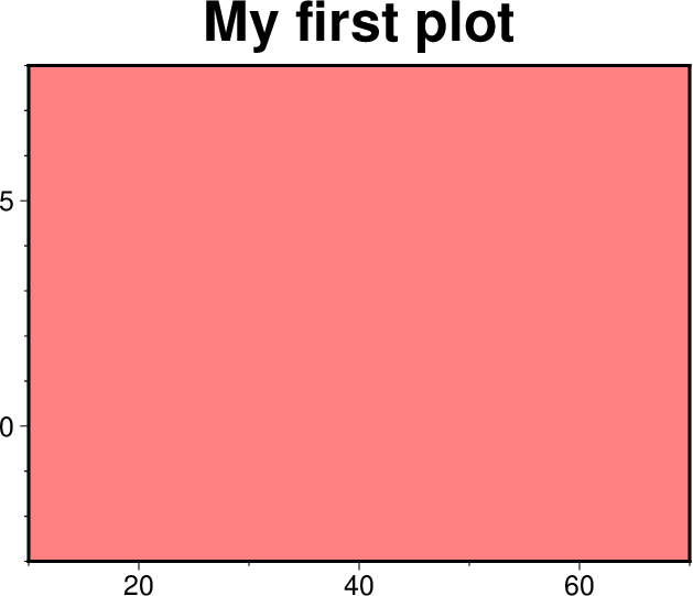
Result of GMT Tutorial example 1.
Exercises:
Try change the proj=:linear values.
Try change the frame values.
Change title and canvas color.
Logarithmic projection
We next will show how to do a basemap for a log–log plot. We have no data set yet but we will imagine that the raw x data range from 3 to 9613 and that y ranges from 10^20 to 10^24. One possibility is
basemap(region=(1,10000,1e20,1e25), proj=:loglog, figsize=(12,8), xaxis=(annot=2, label="Wavelength (m)"),
        yaxis=(annot=1, ticks=3, scale=:pow, label="Power (W)"), frame=(axes=:WS,), show=true)
Make sure your plot looks like our example 2 below
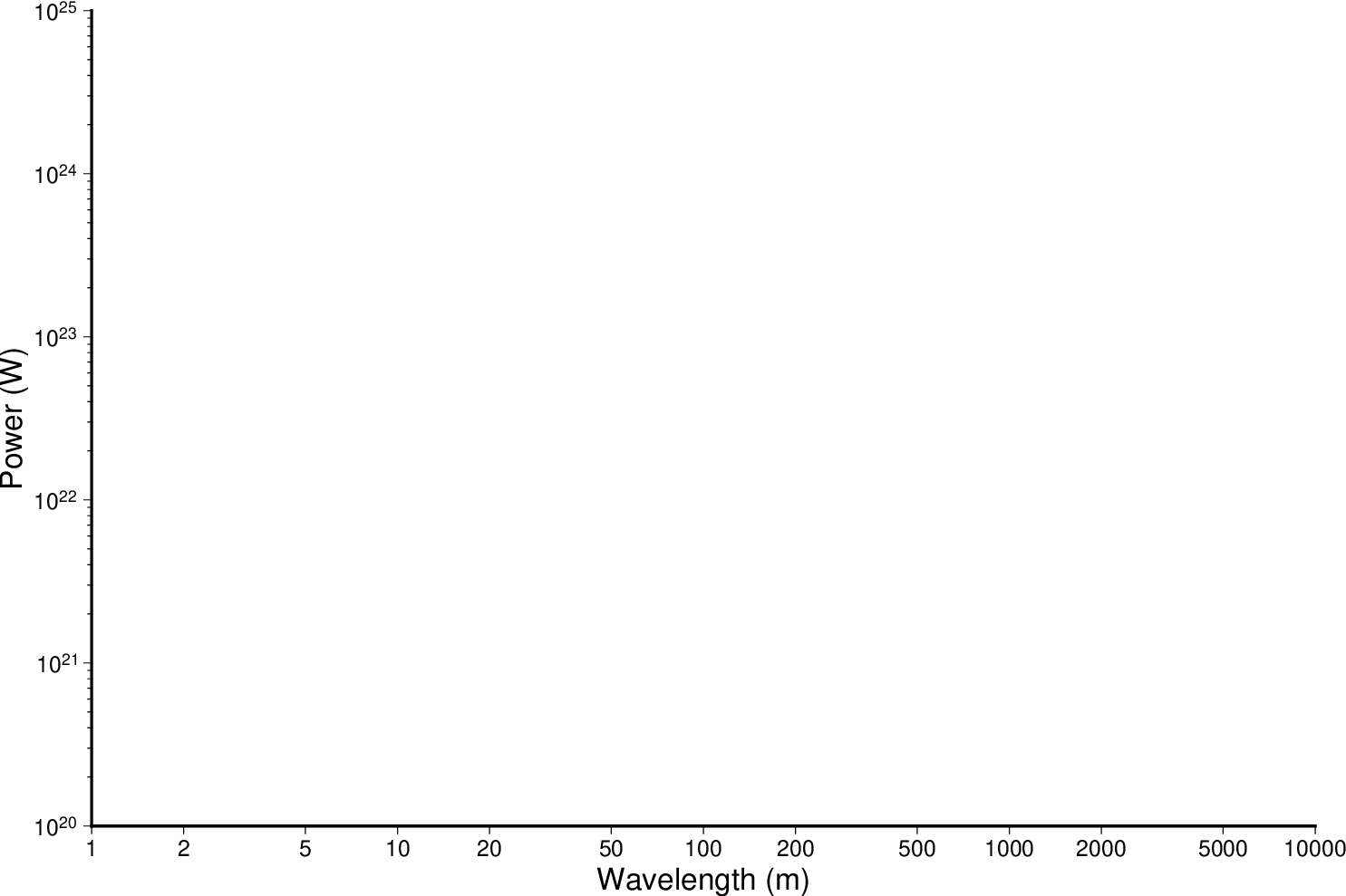
Result of GMT Tutorial example 2.
Exercises:
Do not use proj=:loglog the axes lengths.
Leave the scale=:pow out of the frame string.
Add grid=3 to xaxis and yaxis settings.
Mercator projection
Despite the problems of extreme horizontal exaggeration at high latitudes, the conformal Mercator projection (proj=:merc) remains the stalwart of location maps used by scientists. It is one of several cylindrical projections offered by GMT; here we will only have time to focus on one such projection. The complete syntax is simply
proj=:merc
To make coastline maps we use basemap which automatically will access the GMT coastline, river and border data base derived from the GSHHG database [See Wessel and Smith, 1996]. In addition to the common switches we may need to use some of several coast-specific options:
Option |
Purpose |
|---|---|
area |
Exclude small features or those of high hierarchical levels (see GSHHG.) |
resolution |
Select data resolution (full, high, intermediate, low, or crude) |
land |
Set color of dry areas (default does not paint) |
rivers |
Draw rivers (chose features from one or more hierarchical categories) |
map_scale |
Plot map scale (length scale can be km, miles, or nautical miles) |
borders |
Draw political borders (including US state borders) |
ocean |
Set color for wet areas (default does not paint) |
shore |
Draw coastlines and set pen thickness |
One of shore, land, ocean must be selected. Our first coastline example is from Latin America:
coast(region=(-90,-70,0,20), proj=:merc, land=:chocolate, show=true)
Your plot should look like our example 3 below

Result of GMT Tutorial example 3.
Exercises:
Add the verbose option.
Try region=(270,290,0,20) instead. What happens to the annotations?
Edit your gmt.conf file, change FORMAT_GEO_MAP to another setting (see the gmt.conf documentation), and plot again.
Pick another region and change land color.
Pick a region that includes the north or south poles.
Try shore=”0.25p” instead of (or in addition to) land.
Albers projection
The Albers projection (poj=:albers) is an equal-area conical projection; its conformal cousin is the Lambert conic projection (proj=:lambert). Their usages are almost identical so we will only use the Albers here. The general syntax is
proj=(name=:albers, center=(lon_0,lat_0), parallels=(lat_1,lat_2))
where (lon_0, lat_0) is the map (projection) center and lat_1, lat_2 are the two standard parallels where the cone intersects the Earth’s surface. We try the following command:
coast(region=(-130,-70,24,52), proj=(name=:albers, center=(-100,35), parallels=(33,45)),
      title="Conic Projection", borders=((type=1, pen=:thicker), (type=2, pen=:thinnest)),
      area=500, land=:gray, coast=:thinnest, show=true)
Your plot should look like our example 4 below
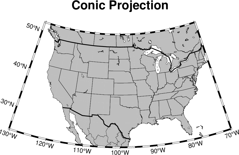
Result of GMT Tutorial example 4.
Exercises:
Change the parameter MAP_GRID_CROSS_SIZE_PRIMARY to make grid crosses instead of gridlines.
Change region to a rectangular box specification instead of minimum and maximum values.
Orthographic projection
The azimuthal orthographic projection (proj=:ortho) is one of several projections with similar syntax and behavior; the one we have chosen mimics viewing the Earth from space at an infinite distance; it is neither conformal nor equal-area. The syntax for this projection is
proj=(name=:ortho, center=(lon_0,lat_0))
where (lon_0, lat_0) is the center of the map (projection). As an example we will try
coast(region=:global360, proj=(name=:ortho, center=(280,30)), frame=(annot=:a, grid=:a),
      area=5000, land=:white, ocean=:DarkTurquoise, show=true)
Your plot should look like our example 5 below
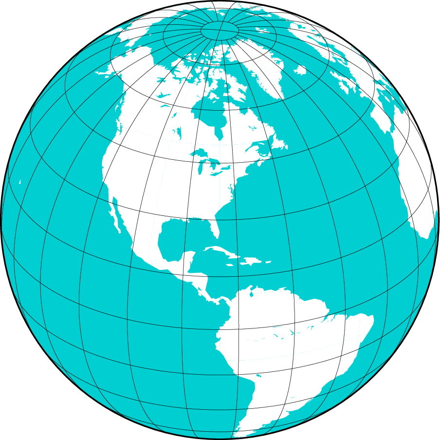
Result of GMT Tutorial example 5
Exercises:
Use the rectangular option in region to make a rectangular map showing the US only.
Eckert IV and VI projection
We conclude the survey of map projections with the Eckert IV and VI projections, two of several projections used for global thematic maps; They are both equal-area projections whose syntax is
proj=(name=:EckertIV, center=lon_0) proj=(name=:EckertVI, center=lon_0)
The lon_0 is the central meridian (which takes precedence over the mid-value implied by the region setting). A simple Eckert VI world map is thus generated by
coast(region=:global360, proj=(name=:EckertVI, center=180), frame=(annot=:a, grid=:a), resolution=:crude,
      area=5000, land=:chocolate, shore=:thinnest, ocean=:DarkTurquoise, show=true)
Your plot should look like our example 6 below
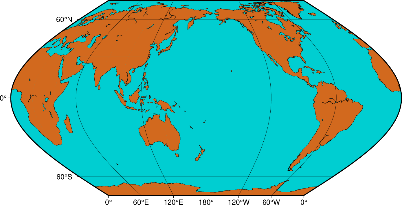
Result of GMT Tutorial example 6
Exercises:
Center the map on Greenwich.
Add a map scale with map_scale.