(25) Global distribution of antipodes

As promised in Example (23) All great-circle paths lead to Rome, we will study antipodes. The antipode of a point at \((\phi, \lambda)\) is the point at \((-\phi, \lambda + 180)\). We seek an answer to the question that has plagued so many for so long: Given the distribution of land and ocean, how often is the antipode of a point on land also on land? And what about marine antipodes? We use grdlandmask and grdmath to map these distributions and calculate the area of the Earth (in percent) that goes with each of the three possibilities. To make sense of our grdmath equations below, note that we first calculate a grid that is +1 when a point and its antipode is on land, -1 if both are in the ocean, and 0 elsewhere. We then seek to calculate the area distribution of dry antipodes by only pulling out the nodes that equal +1. As each point represent an area approximated by \(\Delta \phi \times \Delta \lambda\) where the \(\Delta \lambda\) term’s actual dimension depends on \(\cos (\phi)\), we need to allow for that shrinkage, normalize our sum to that of the whole area of the Earth, and finally convert that ratio to percent. Since the \(\Delta \lambda\), \(\Delta \phi\) terms appear twice in these expressions they cancel out, leaving the somewhat intractable expressions below where the sum of \(\cos (\phi)\) for all \(\phi\) is known to equal \(2N_y / \pi\):

In the end we obtain a funny-looking map depicting the antipodal distribution as well as displaying in legend form the requested percentages. Note that the script is set to evaluate a global 30 minute grid for expediency (D = 30), hence several smaller land masses that do have terrestrial antipodes do not show up. If you want a more accurate map you can set the parameter D to a smaller increment (try 5 and wait a few minutes).

The call to grdimage includes the -Sn to suspend interpolation and only return the value of the nearest neighbor. This option is particularly practical for plotting categorical data, like these, that should not be interpolated.

#!/usr/bin/env bash
#		GMT EXAMPLE 25
#
# Purpose:	Display distribution of antipode types
# GMT modules:	set, grdlandmask, grdmath, grd2xyz, math, grdimage, coast, legend
# Unix progs:	rm
#
# Create D minutes global grid with -1 over oceans and +1 over land
gmt begin ex25
	D=30
	gmt grdlandmask -Rg -I${D}m -Dc -A500 -N-1/1/1/1/1 -r -Gwetdry.nc
	# Manipulate so -1 means ocean/ocean antipode, +1 = land/land, and 0 elsewhere
	gmt grdmath -fg wetdry.nc DUP 180 ROTX FLIPUD ADD 2 DIV = key.nc
	# Calculate percentage area of each type of antipode match.
	gmt grdmath -Rg -I${D}m -r Y COSD 60 $D DIV 360 MUL DUP MUL PI DIV DIV 100 MUL = scale.nc
	gmt grdmath key.nc -1 EQ 0 NAN scale.nc MUL = tmp.nc
	gmt grd2xyz tmp.nc -s -ZTLf > key.b
	ocean=$(gmt math -bi1f -Ca -S key.b SUM UPPER RINT =)
	gmt grdmath key.nc 1 EQ 0 NAN scale.nc MUL = tmp.nc
	gmt grd2xyz tmp.nc -s -ZTLf > key.b
	land=$(gmt math -bi1f -Ca -S key.b SUM UPPER RINT =)
	gmt grdmath key.nc 0 EQ 0 NAN scale.nc MUL = tmp.nc
	gmt grd2xyz tmp.nc -s -ZTLf > key.b
	mixed=$(gmt math -bi1f -Ca -S key.b SUM UPPER RINT =)
	# Generate corresponding color table
	gmt makecpt -Cblue,gray,red -T-1.5/1.5/1 -N
	# Create the final plot and overlay coastlines
	gmt set FONT_ANNOT_PRIMARY +10p FORMAT_GEO_MAP dddF
	gmt grdimage key.nc -JKs180/22c -Bx60 -By30 -BWsNE+t"Antipodal comparisons" -nn
	gmt coast -Wthinnest -Dc -A500
	# Place an explanatory legend below
	gmt legend -DJBC+w15c -Y-0.5c -F+pthick <<- END
	N 3
	S 0.4c s 0.5c red  0.25p 0.75c Terrestrial Antipodes [$land %]
	S 0.4c s 0.5c blue 0.25p 0.75c Oceanic Antipodes [$ocean %]
	S 0.4c s 0.5c gray 0.25p 0.75c Mixed Antipodes [$mixed %]
	END
	rm -f *.nc key.*
gmt end show

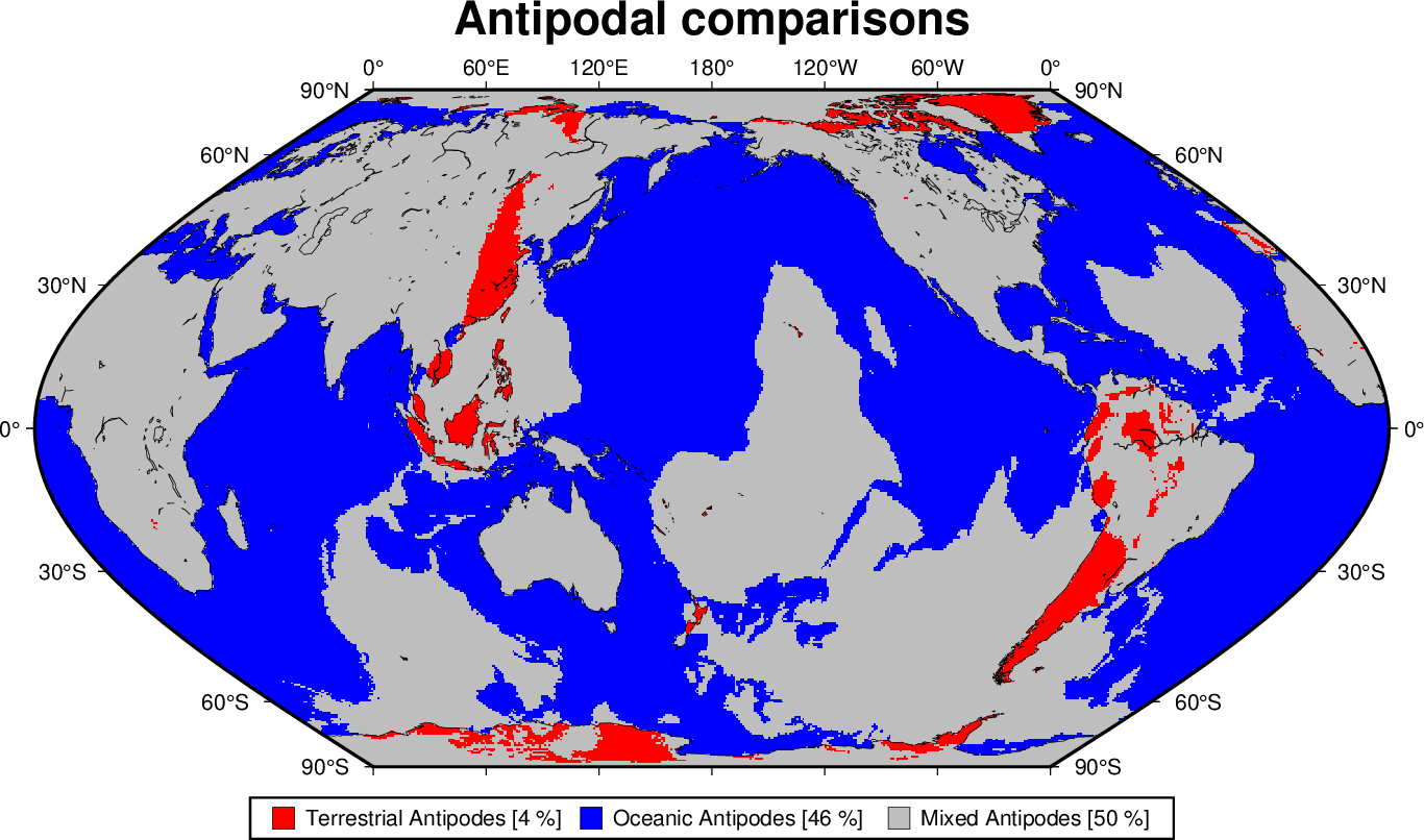
Global distribution of antipodes.