gmtregress¶

Linear regression of 1-D data sets

Synopsis¶

gmt regress [ table ] [ -A[min/max/inc][+f[n|p]] ] [ -Clevel ] [ -Ex|y|o|r ] [ -Fflags ] [ -N1|2|r|w ] [ -S[r] ] [ -T[min/max/]inc[+i|n] |-Tfile|list ] [ -V[level] ] [ -W[w][x][y][r] ] [ -Z[±]limit ] [ -aflags ] [ -bbinary ] [ -d[+ccol]nodata ] [ -eregexp ] [ -fflags ] [ -ggaps ] [ -hheaders ] [ -iflags ] [ -oflags ] [ -qflags ] [ -sflags ] [ -wflags ] [ --PAR=value ]

Note: No space is allowed between the option flag and the associated arguments.

Description¶

regress reads one or more data tables [or stdin] and determines the best linear [weighted] regression model \(y(x) = a + b x\) for each segment using the chosen parameters. The user may specify which data and model components should be reported. By default, the model will be evaluated at the input points, but alternatively you can specify an equidistant range over which to evaluate the model, or turn off evaluation completely. Instead of determining the best fit we can perform a scan of all possible regression lines (for a range of slope angles) and examine how the chosen misfit measure varies with slope. This is particularly useful when analyzing data with many outliers. Note: If you actually need to work with \(\log_{10}\) of x or y you can accomplish that transformation during the read phase by using the -i option.

Required Arguments¶

table: One or more ASCII (or binary, see -bi[ncols][type]) data table file(s) holding a number of data columns. If no tables are given then we read from standard input. The first two columns are expected to contain the required x and y data. Depending on your -W and -E settings we may expect an additional 1-3 columns with error estimates of one of both of the data coordinates, and even their correlation (see -W for details).

Optional Arguments¶

-A[min/max/inc][+f[n|p]]: There are two uses for this setting: (1) Instead of determining a best-fit regression we explore the full range of regressions. Examine all possible regression lines with slope angles between min and max, using steps of inc degrees [-90/+90/1]. For each slope, the optimum intercept is determined based on your regression type (-E) and misfit norm (-N) settings. For each data segment we report the four columns angle, E, slope, intercept, for the range of specified angles. The best model parameters within this range are written into the segment header and reported in verbose information mode (-Vi). (2) Except for -N2, append +f to force the best regression to only consider the given restricted range of angles [all angles]. As shortcuts for negative or positive slopes, just use +fn or +fp, respectively.

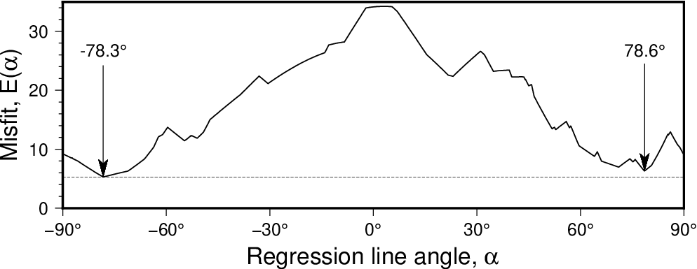
_images/GMT_slopes.png — Scanning slopes (-A) to see how the misfit for an fully orthogonal regression using the LMS (**-Nr**) criterion varies with the line angle. Here we see the best solution gives a line angle of -78.3 degrees but there is another local minimum for an angle of 78.6 degrees that is almost as good.¶

-Clevel: Set the confidence level (in %) to use for the optional calculation of confidence bands on the regression [95]. This is only used if -F includes the output column c.

-Ex|y|o|r: Type of linear regression, i.e., select the type of misfit we should calculate. Choose from x (regress x on y; i.e., the misfit is measured horizontally from data point to regression line), y (regress y on x; i.e., the misfit is measured vertically [Default]), o (orthogonal regression; i.e., the misfit is measured from data point orthogonally to nearest point on the line), or r (Reduced Major Axis regression; i.e., the misfit is the product of both vertical and horizontal misfits) [y].

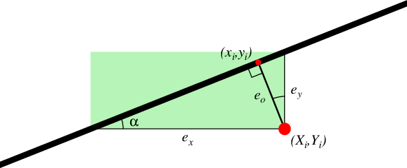
_images/GMT_misfit.png — The four types of misfit. The sum of the squared lengths of \(e_k\) is minimized, for k = x, y, or o. For **-Er** the sum of the green areas is minimized instead.¶

-Fflags: Append a combination of the columns you wish returned; the output order will match the order specified. Choose from x (observed x), y (observed y), m (model prediction), r (residual = data minus model), c (symmetrical confidence interval on the regression; see -C for specifying the level), z (standardized residuals or so-called z-scores) and w (outlier weights 0 or 1; for -Nw these are the Reweighted Least Squares weights) [xymrczw]. As an alternative to evaluating the model, just give -Fp and we instead write a single record with the 12 model parameters npoints xmean ymean angle misfit slope intercept sigma_slope sigma_intercept r R n_effective. Note: R is only set when -Ey is selected.

-N1|2|r|w: Selects the norm to use for the misfit calculation. Choose among 1 (\(L_1\) measure; the mean of the absolute residuals), 2 (Least-squares; the mean of the squared residuals), r (LMS; The least median of the squared residuals), or w (RLS; Reweighted Least Squares: the mean of the squared residuals after outliers identified via LMS have been removed) [Default is 2]. Traditional regression uses \(L_2\) while \(L_1\) and in particular LMS are more robust in how they handle outliers. As alluded to, RLS implies an initial LMS regression which is then used to identify outliers in the data, assign these a zero weight, and then redo the regression using a \(L_2\) norm.

-S[r]: Restricts which records will be output. By default all data records will be output in the format specified by -F. Use -S to exclude data points identified as outliers by the regression. Alternatively, use -Sr to reverse this and only output the outlier records.

-T[min/max/]inc[+i|n] |-Tfile|list: Evaluate the best-fit regression model at the equidistant points implied by the arguments. If only -Tinc is given instead we will reset min and max to the extreme x-values for each segment. To skip the model evaluation entirely, simply provide -T0. For details on array creation, see Generate 1D Array.

-V[level]: Select verbosity level [w]. (See full description) (See cookbook information).

-W[w][x][y][r]: Specifies weighted regression and which weights will be provided. Append x if giving one-\(\sigma\) uncertainties in the x-observations, y if giving one-\(\sigma\) uncertainties in y, and r if giving correlations between x and y observations, in the order these columns appear in the input (after the two required and leading x, y columns). Giving both x and y (and optionally r) implies an orthogonal regression, otherwise giving x requires -Ex and y requires -Ey. We convert uncertainties in x and y to regression weights w via the relationship \(w = 1/\sigma\). Use -Ww if the we should interpret the input columns to have precomputed weights instead. Note: Residuals with respect to the regression line will be scaled by the given weights. Most norms will then square this weighted residual (-N1 is the only exception).

-Z[±]limit: Change the threshold for outlier detection: When -Nw is used, residual z-scores that exceed this limit [±2.5] will be flagged as outliers. To only consider negative or positive z-scores as possible outliers, specify a signed limit.

-a[[col=]name[,…]] (more …): Set aspatial column associations col=name.

-birecord[+b|l] (more …): Select native binary format for primary table input.

-borecord[+b|l] (more …): Select native binary format for table output. [Default is same as input].

-d[i|o][+ccol]nodata (more …): Replace input columns that equal nodata with NaN and do the reverse on output.

-e[~]“pattern” | -e[~]/regexp/[i] (more …): Only accept data records that match the given pattern.

-f[i|o]colinfo (more …): Specify data types of input and/or output columns.

-gx|y|z|d|X|Y|Dgap[u][+a][+ccol][+n|p] (more …): Determine data gaps and line breaks.

-h[i|o][n][+c][+d][+msegheader][+rremark][+ttitle] (more …): Skip or produce header record(s).

-icols[+l][+ddivisor][+sscale|d|k][+ooffset][,…][,t[word]] (more …): Select input columns and transformations (0 is first column, t is trailing text, append word to read one word only).

-ocols[,…][,t[word]] (more …): Select output columns (0 is first column; t is trailing text, append word to write one word only).

-q[i|o][~]rows|limits[+ccol][+a|f|s] (more …): Select input or output rows or data limit(s) [all].

-s[cols][+a][+r] (more …): Set handling of NaN records for output.

-wy|a|w|d|h|m|s|cperiod[/phase][+ccol] (more …): Convert an input coordinate to a cyclical coordinate.

-^ or just -: Print a short message about the syntax of the command, then exit (NOTE: on Windows just use -).
-+ or just +: Print an extensive usage (help) message, including the explanation of any module-specific option (but not the GMT common options), then exit.
-? or no arguments: Print a complete usage (help) message, including the explanation of all options, then exit.
--PAR=value: Temporarily override a GMT default setting; repeatable. See gmt.conf for parameters.

ASCII Format Precision¶

The ASCII output formats of numerical data are controlled by parameters in your gmt.conf file. Longitude and latitude are formatted according to FORMAT_GEO_OUT, absolute time is under the control of FORMAT_DATE_OUT and FORMAT_CLOCK_OUT, whereas general floating point values are formatted according to FORMAT_FLOAT_OUT. Be aware that the format in effect can lead to loss of precision in ASCII output, which can lead to various problems downstream. If you find the output is not written with enough precision, consider switching to binary output (-bo if available) or specify more decimals using the FORMAT_FLOAT_OUT setting.

Generate 1D Array¶

We will demonstrate the use of options for creating 1-D arrays via gmtmath. Make an evenly spaced coordinate array from min to max in steps of inc, e.g.,:

gmt math -o0 -T3.1/4.2/0.1 T =
1
2
3
4
5
6
7

Append +b if we should take log2 of min and max, get their nearest integers, build an equidistant log2-array using inc integer increments in log2, then undo the log2 conversion. E.g., -T3/20/1+b will produce this sequence:

gmt math -o0 -T3/20/1+b T =
4
8
16

Append +l if we should take log10 of min and max and build an array where inc can be 1 (every magnitude), 2, (1, 2, 5 times magnitude) or 3 (1-9 times magnitude). E.g., -T7/135/2+l will produce this sequence:

gmt math -o0 -T7/135/2+l T =
10
20
50
100

For output values less frequently than every magnitude, use a negative integer inc:

gmt math -o0 -T1e-4/1e4/-2+l T =
0.0001
0.01
1
100
10000

Append +i if inc is a fractional number and it is cleaner to give its reciprocal value instead. To set up times for a 24-frames per second animation lasting 1 minute, run:

gmt math -o0 -T0/60/24+i T =
0
0.0416666666667
0.0833333333333
0.125
0.166666666667
...

Append +n if inc is meant to indicate the number of equidistant coordinates instead. To have exactly 5 equidistant values from 3.44 and 7.82, run:

gmt math -o0 -T3.44/7.82/5+n T =
44
535
63
725
82

Alternatively, let inc be a file with output coordinates in the first column, or provide a comma-separated list of specific coordinates, such as the first 6 Fibonacci numbers:

gmt math -o0 -T0,1,1,2,3,5 T =
0
1
1
2
3
5

Note: Should you need to ensure that the coordinates are unique and sorted (in case the file or list are not sorted or have duplicates) then supply the +u modifier.

If you only want a single value then you must append a comma to distinguish the list from the setting of an increment.

If the module allows you to set up an absolute time series, append a valid time unit from the list year, month, day, hour, minute, and second to the given increment; add +t to ensure time column (or use -f). Note: The internal time unit is still controlled independently by TIME_UNIT. The first 7 days of March 2020:

gmt math -o0 -T2020-03-01T/2020-03-07T/1d T =
2020-03-01T00:00:00
2020-03-02T00:00:00
2020-03-03T00:00:00
2020-03-04T00:00:00
2020-03-05T00:00:00
2020-03-06T00:00:00
2020-03-07T00:00:00

A few modules allow for +a which will paste the coordinate array to the output table.

Likewise, if the module allows you to set up a spatial distance series (with distances computed from the first two data columns), specify a new increment as inc with a geospatial distance unit from the list degree (arc), minute (arc), second (arc), meter, foot, kilometer, Miles (statute), nautical miles, or survey foot; see -j for calculation mode. To interpolate Cartesian distances instead, you must use the special unit c.

Finally, if you are only providing an increment and will obtain min and max from the data, then it is possible (max - min)/inc is not an integer, as required. If so, then inc will be adjusted to fit the range. Alternatively, append +e to keep inc exact and adjust max instead (keeping min fixed).

Notes:¶

The output segment header will contain all the various statistics we compute for each segment. These are in order: N (number of points), x0 (weighted mean x), y0 (weighted mean y), angle (of line), E (misfit), slope, intercept, sigma_slope, and sigma_intercept. For the standard regression (-Ey) we also report the Pearsonian correlation (r) and coefficient of determination (R). We end with the effective number of measurements, \(n_{eff}\).

For weighted data and the calculation of squared regression misfit to minimize (-N2), we use

\[E_2(\nu) = \frac{\sum_{i=1}^n w_i e_i^2}{\sum_{i=1}^n w_i} \frac{n_{eff}}{n_{eff}-2},\]

where the effective number of measurements is given by

\[n_{eff} = \frac{\left (\sum_{i=1}^n w_i\right )^2}{\sum_{i=1}^n w_i^2}.\]

and hence \(\nu = n_{eff} - 2\) are the effective degrees of freedom.

Examples¶

Note: Below are some examples of valid syntax for this module. The examples that use remote files (file names starting with @) can be cut and pasted into your terminal for testing. Other commands requiring input files are just dummy examples of the types of uses that are common but cannot be run verbatim as written.

To return the coordinates on the best-fit orthogonal regression line through the data in the remote file hertzsprung-russell.txt, try:

gmt regress @hertzsprung-russell.txt -Eo -Fxm

To do a standard least-squares regression on the x-y data in points.txt and return x, y, and model prediction with 99% confidence intervals, try

gmt regress points.txt -Fxymc -C99 > points_regressed.txt

To just get the slope for the above regression, try

slope=`gmt regress points.txt -Fp -o5`

To do a reweighted least-squares regression on the data rough.txt and return x, y, model prediction and the RLS weights, try

gmt regress rough.txt -Fxymw > points_regressed.txt

To do an orthogonal least-squares regression on the data crazy.txt but first take the logarithm of both x and y, then return x, y, model prediction and the normalized residuals (z-scores), try

gmt regress crazy.txt -Eo -Fxymz -i0-1l > points_regressed.txt

To examine how the orthogonal LMS misfits vary with angle between 0 and 90 in steps of 0.2 degrees for the same file, try

gmt regress points.txt -A0/90/0.2 -Eo -Nr > points_analysis.txt

To force an orthogonal LMS to pick the best solution with a positive slope, try

gmt regress points.txt -A+fp -Eo -Nr > best_pos_slope.txt

References¶

Bevington, P. R., 1969, Data reduction and error analysis for the physical sciences, 336 pp., McGraw-Hill, New York.

Draper, N. R., and H. Smith, 1998, Applied regression analysis, 3rd ed., 736 pp., John Wiley and Sons, New York.

Rousseeuw, P. J., and A. M. Leroy, 1987, Robust regression and outlier detection, 329 pp., John Wiley and Sons, New York.

York, D., N. M. Evensen, M. L. Martinez, and J. De Basebe Delgado, 2004, Unified equations for the slope, intercept, and standard errors of the best straight line, Am. J. Phys., 72(3), 367-375.