psvelo
Plot velocity vectors, crosses, anisotropy bars and wedges
Synopsis
gmt psvelo [ table ] -Jparameters -Rregion -Sformat[scale][/args][+ffont] [ -Aparameters ] [ -B[p|s]parameters ] [ -Ccpt] [ -Efill ] [ -Gfill ] [ -H[scale] ] [ -I[intens] ] [ -K ] [ -L[pen[+c[f|l]]] ] [ -N ] [ -O ] [ -P ] [ -U[stamp] ] [ -V[level] ] [ -W[pen][+c[f|l]] ] [ -X[a|c|f|r][xshift] ] [ -Y[a|c|f|r][yshift] ] [ -Z[m|e|n|u][+e] ] [ -dinodata ] [ -eregexp ] [ -hheaders ] [ -iflags ] [ -pflags ] [ -qiflags ] [ -ttransp ] [ -:[i|o] ] [ --PAR=value ]
Note: No space is allowed between the option flag and the associated arguments.
Description
Reads data values from files [or standard input] and will plot the selected geodesy symbol on a map. You may choose from velocity vectors and their uncertainties, rotational wedges and their uncertainties, anisotropy bars, or strain crosses. Symbol fills or their outlines may be colored based on constant parameters or via color lookup tables.
Required Arguments
- table
One or more ASCII (or binary, see -bi[ncols][type]) data table file(s) holding a number of data columns. If no tables are given then we read from standard input.
- -Jparameters
Specify the projection. (See full description) (See cookbook summary) (See projections table).
- -Rwest/east/south/north[/zmin/zmax][+r][+uunit]
west, east, south, and north specify the region of interest, and you may specify them in decimal degrees or in [±]dd:mm[:ss.xxx][W|E|S|N] format Append +r if lower left and upper right map coordinates are given instead of w/e/s/n. The two shorthands -Rg and -Rd stand for global domain (0/360 and -180/+180 in longitude respectively, with -90/+90 in latitude). Set geographic regions by specifying ISO country codes from the Digital Chart of the World using -Rcode1,code2,…[+r|R[incs]] instead: Append one or more comma-separated countries using the 2-character ISO 3166-1 alpha-2 convention. To select a state of a country (if available), append .state, e.g, US.TX for Texas. To specify a whole continent, prepend = to any of the continent codes AF (Africa), AN (Antarctica), AS (Asia), EU (Europe), OC (Oceania), NA (North America), or SA (South America). Use +r to modify the bounding box coordinates from the polygon(s): Append inc, xinc/yinc, or winc/einc/sinc/ninc to adjust the region to be a multiple of these steps [no adjustment]. Alternatively, use +R to extend the region outward by adding these increments instead, or +e which is like +r but it ensures that the bounding box extends by at least 0.25 times the increment [no extension]. Alternatively for grid creation, give Rcodelon/lat/nx/ny, where code is a 2-character combination of L, C, R (for left, center, or right) and T, M, B for top, middle, or bottom. e.g., BL for lower left. This indicates which point on a rectangular region the lon/lat coordinate refers to, and the grid dimensions nx and ny with grid spacings via -I is used to create the corresponding region. Alternatively, specify the name of an existing grid file and the -R settings (and grid spacing and registration, if applicable) are copied from the grid. Appending +uunit expects projected (Cartesian) coordinates compatible with chosen -J and we inversely project to determine actual rectangular geographic region. For perspective view (-p), optionally append /zmin/zmax. In case of perspective view (-p), a z-range (zmin, zmax) can be appended to indicate the third dimension. This needs to be done only when using the -Jz option, not when using only the -p option. In the latter case a perspective view of the plane is plotted, with no third dimension.
- -S
Selects the meaning of the columns in the data file and the figure to be plotted. In all cases, the scales are in data units per length unit and sizes are in length units (default length unit is controlled by PROJ_LENGTH_UNIT unless c, i, or p is appended).
-Se[velscale/]confidence[+ffont]
Velocity ellipses in (N,E) convention. The velscale sets the scaling of the velocity arrows. If velscale is not given the we read it from the data file as an extra column. The confidence sets the 2-dimensional confidence limit for the ellipse, e.g., 0.95 for 95% confidence ellipse. Use +f to set the font and size of the text [9p,Helvetica,black]; give +f0 to deactivate labeling. The arrow will be drawn with the pen attributes specified by the -W option and arrow-head can be colored via -G. The ellipse will be filled with the color or shade specified by the -E option [default is transparent], and its outline will be drawn if -L is selected using the pen selected (by -W if not given by -L). Parameters are expected to be in the following columns:
1,2: longitude, latitude of station (-: option interchanges order) 3,4: eastward, northward velocity (-: option interchanges order) 5,6: uncertainty of eastward, northward velocities (1-sigma) (-: option interchanges order) 7: correlation between eastward and northward components Trailing text: name of station (optional).
-Sn[barscale]
Anisotropy bars. The barscale sets the scaling of the bars. If barscale is not given the we read it from the data file as an extra column. Parameters are expected to be in the following columns:
1,2: longitude, latitude of station (-: option interchanges order) 3,4: eastward, northward components of anisotropy vector (-: option interchanges order)
-Sr[velscale/]confidence[+ffont]
Velocity ellipses in rotated convention. The velscale sets the scaling of the velocity arrows. If velscale is not given the we read it from the data file as an extra column. The confidence sets the 2-dimensional confidence limit for the ellipse, e.g., 0.95 for 95% confidence ellipse. Use +f to set the font and size of the text [9p,Helvetica,black]; give +f0 to deactivate labeling. The arrow will be drawn with the pen attributes specified by the -W option and arrow-head can be colored via -G. The ellipse will be filled with the color or shade specified by the -E option [default is transparent], and its outline will be drawn if -L is selected using the pen selected (by -W if not given by -L). Parameters are expected to be in the following columns:
1,2: longitude, latitude, of station (-: option interchanges order) 3,4: eastward, northward velocity (-: option interchanges order) 5,6: semi-major, semi-minor axes 7: counter-clockwise angle, in degrees, from horizontal axis to major axis of ellipse. Trailing text: name of station (optional)
-Sw[wedgescale/]wedgemag
Rotational wedges. The wedgescale sets the size of the wedges. If wedgescale is not given the we read it from the data file as an extra column. Rotation values are multiplied by wedgemag before plotting. For example, setting wedgemag to 1.e7 works well for rotations of the order of 100 nanoradians/yr. Use -G to set the fill color or shade for the wedge, and -E to set the color or shade for the uncertainty. Parameters are expected to be in the following columns:
1,2: longitude, latitude, of station (-: option interchanges order) 3: rotation in radians 4: rotation uncertainty in radians
-Sx[cross_scale]
gives Strain crosses. The cross_scale sets the size of the cross. If cross_scale is not given the we read it from the data file as an extra column. Parameters are expected to be in the following columns:
1,2: longitude, latitude, of station (-: option interchanges order) 3: eps1, the most extensional eigenvalue of strain tensor, with extension taken positive. 4: eps2, the most compressional eigenvalue of strain tensor, with extension taken positive. 5: azimuth of eps2 in degrees CW from North.
Optional Arguments
- -Aparameters
Modify vector parameters. For vector heads, append vector head size [Default is 9p]. See Vector Attributes for specifying additional attributes.
- -B[p|s]parameters
Set map boundary frame and axes attributes. (See full description) (See cookbook information).
- -Ccpt
Give a CPT and let symbol color normally set by -G be determined from the magnitude. See -Z for other selections.
- -DSigma_scale
can be used to rescale the uncertainties of velocities (-Se and -Sr) and rotations (-Sw). Can be combined with the confidence variable.
- -Efill (more …)
Sets the color or shade used for filling uncertainty wedges (-Sw) or velocity error ellipses (-Se or -Sr). If -E is not specified, the uncertainty regions will be transparent. Note: Using -C and -Z+e will update the uncertainty fill color based on the selected measure in -Z [magnitude error].
- -Gfill (more …)
Select color or pattern for filling of symbols [Default is no fill]. Note: Using -C (and optionally -Z) will update the symbol fill color based on the selected measure in -Z [magnitude].
- -H[scale]
Scale symbol sizes and pen widths on a per-record basis using the scale read from the data set, given as the first column after the (optional) z and size columns [no scaling]. The symbol size is either provided by -S or via the input size column. Alternatively, append a constant scale that should be used instead of reading a scale column.
- -Iintens
Use the supplied intens value (nominally in the -1 to +1 range) to modulate the symbol fill color by simulating illumination [none]. If no intensity is provided we will instead read intens from an extra data column after the required input columns determined by -S.
- -L[pen[+c[f|l]]]
Draw lines. Ellipses and rotational wedges will have their outlines drawn using current pen (see -W). Alternatively, append a separate pen to use for the error outlines. If the modifier +cl is appended then the color of the pen are updated from the CPT (see -C). If instead modifier +cf is appended then the color from the cpt file is applied to error fill only [Default]. Use just +c to set both pen and fill color.
- -N
Do NOT skip symbols that fall outside the frame boundary specified by -R. [Default plots symbols inside frame only].
- -U[label|+c][+jjust][+odx/dy]
Draw GMT time stamp logo on plot. (See full description) (See cookbook information).
- -V[level]
Select verbosity level [w]. (See full description) (See cookbook information).
- -W[pen][+c[f|l]]
Set pen attributes for velocity arrows, ellipse circumference and fault plane edges. [Defaults: width = default, color = black, style = solid]. If the modifier +cl is appended then the color of the pen are updated from the CPT (see -C). If instead modifier +cf is appended then the color from the cpt file is applied to symbol fill only [Default]. Use just +c to set both pen and fill color.
- -X[a|c|f|r][xshift]
Shift plot origin. (See full description) (See cookbook information).
- -Y[a|c|f|r][yshift]
Shift plot origin. (See full description) (See cookbook information).
- Z[m|e|n|u][+e]
Select the quantity that will be used with the CPT given via -C to set the fill color. Choose from magnitude (vector magnitude or rotation magnitude), east-west velocity, north-south velocity, or user-supplied data column (supplied after the required columns). To instead use the corresponding error estimates (i.e., vector or rotation uncertainty) to lookup the color and paint the error ellipse or wedge instead, append +e.
- -dinodata (more …)
Replace input columns that equal nodata with NaN.
- -e[~]“pattern” | -e[~]/regexp/[i] (more …)
Only accept data records that match the given pattern.
- -h[i|o][n][+c][+d][+msegheader][+rremark][+ttitle] (more …)
Skip or produce header record(s).
- -icols[+l][+ddivide][+sscale][+ooffset][,…][,t[word]] (more …)
Select input columns and transformations (0 is first column, t is trailing text, append word to read one word only).
- -p[x|y|z]azim[/elev[/zlevel]][+wlon0/lat0[/z0]][+vx0/y0] (more …)
Select perspective view.
- -qi[~]rows[+ccol][+a|f|s] (more …)
Select input rows or data range(s) [default is all rows].
- -t[transp[/transp2]][+f][+s]
Set transparency level for an overlay, in [0-100] percent range. [Default is 0, i.e., opaque]. Only visible when PDF or raster format output is selected. Only the PNG format selection adds a transparency layer in the image (for further processing). If given, transp applies to both fill and stroke, but you can limit the transparency to one of them by appending +f or +s for fill or stroke, respectively. Alternatively, append /transp2 to set separate transparencies for fills and strokes. If no transparencies are given then we expect to read them from the last numerical column(s). Use the modifiers to indicate which one(s) we should be reading (if both are requested, fill transparency is expected before stroke transparency in the column order). If just -t is given then we interpret it to mean -t+f for fill transparency only.
- -:[i|o] (more …)
Swap 1st and 2nd column on input and/or output.
- -^ or just -
Print a short message about the syntax of the command, then exit (NOTE: on Windows just use -).
- -+ or just +
Print an extensive usage (help) message, including the explanation of any module-specific option (but not the GMT common options), then exit.
- -? or no arguments
Print a complete usage (help) message, including the explanation of all options, then exit.
- --PAR=value
Temporarily override a GMT default setting; repeatable. See gmt.conf for parameters.
Vector Attributes
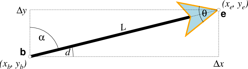
Vector attributes are controlled by options and modifiers. We will refer to this figure and the labels therein when introducing the corresponding modifiers. All vectors require you to specify the begin point \(x_b, y_b\) and the end point \(x_e, y_e\), or alternatively the direction d and length L, while for map projections we usually specify the azimuth \(\alpha\) instead.
Several modifiers may be appended to vector-producing options for specifying the placement of vector heads, their shapes, and the justification of the vector. Below, left and right refers to the side of the vector line when viewed from the beginning point (b) to the end point (e) of a line segment:
+aangle sets the angle \(\theta\) of the vector head apex [30].
+b places a vector head at the beginning of the vector path [none]. Optionally, append t for a terminal line, c for a circle, a for arrow [Default], i for tail, A for plain open arrow, and I for plain open tail. Further append l|r to only draw the left or right half-sides of this head [both sides].
+e places a vector head at the end of the vector path [none]. Optionally, append t for a terminal line, c for a circle, a for arrow [Default], i for tail, A for plain open arrow, and I for plain open tail. Further append l|r to only draw the left or right half-sides of this head [both sides].
+g[fill] sets the vector head fill [Default fill is used, which may be no fill]. Turn off vector head fill by not appending a fill. Some modules have a separate -Gfill option and if used will select the fill as well.
+hshape sets the shape of the vector head (range -2/2). Default is controlled by MAP_VECTOR_SHAPE [default is theme dependent]. A zero value produces no notch (e.g., the dashed line in the figure). Positive values moves the notch toward the head apex while a negative value moves away. The example above uses +h0.5.
+l draws half-arrows, using only the left side of specified heads [both sides].
+m places a vector head at the mid-point the vector path [none]. Append f or r for forward or reverse direction of the vector [forward]. Optionally, append t for a terminal line, c for a circle, a for arrow [Default], i for tail, A for plain open arrow, and I for plain open tail. Further append l|r to only draw the left or right half-sides of this head [both sides]. Cannot be combined with +b or +e.
+nnorm scales down vector attributes (pen thickness, head size) with decreasing length, where vector plot lengths shorter than norm will have their attributes scaled by length/norm [arrow attributes remains invariant to length]. For Cartesian vectors specify a length in plot units, while for geovectors specify a length in km.
+o[plon/plat] specifies the oblique pole for the great or small circles. Only needed for great circles if +q is given. If no pole is appended then we default to the north pole.
+p[pen] sets the vector pen attributes. If no pen is appended then the head outline is not drawn. [Default pen is half the width of stem pen, and head outline is drawn]. Above, we used +p2p,orange. The vector stem attributes are controlled by -W.
+q means the input direction, length data instead represent the start and stop opening angles of the arc segment relative to the given point. See +o to specify a specific pole for the arc [north pole].
+r draws half-arrows, using only the right side of specified heads [both sides].
+t[b|e]trim will shift the beginning or end point (or both) along the vector segment by the given trim; append suitable unit (c, i, or p). If the modifiers b|e are not used then trim may be two values separated by a slash, which is used to specify different trims for the beginning and end. Positive trims will shorted the vector while negative trims will lengthen it [no trim].
In addition, all but circular vectors may take these modifiers:
+jjust determines how the input x,y point relates to the vector. Choose from beginning [default], end, or center.
+s means the input angle, length are instead the \(x_e, y_e\) coordinates of the vector end point.
Finally, Cartesian vectors may take these modifiers:
+zscale expects input \(\Delta x, \Delta y\) vector components and uses the scale to convert to polar coordinates with length in given unit.
Note: Vectors were completely redesigned for GMT5 which separated the vector head (a polygon) from the vector stem (a line). In GMT4, the entire vector was a polygon and it could only be a straight Cartesian vector. Yes, the old GMT4 vector shape remains accessible if you specify a vector (-Sv|V) using the GMT4 syntax, explained here: size, if present, will be interpreted as \(t_w/h_l/h_w\) or tailwidth/headlength/halfheadwidth [Default is 0.075c/0.3c/0.25c (or 0.03i/0.12i/0.1i)]. By default, arrow attributes remain invariant to the length of the arrow. To have the size of the vector scale down with decreasing size, append +nnorm, where vectors shorter than norm will have their attributes scaled by length/norm. To center the vector on the balance point, use -Svb; to align point with the vector head, use -Svh; to align point with the vector tail, use -Svt [Default]. To give the head point’s coordinates instead of direction and length, use -Svs. Upper case B, H, T, S will draw a double-headed vector [Default is single head].
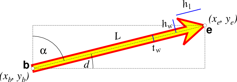
A GMT 4 vector has no separate pen for the stem -- it is all part of a Cartesian polygon. You may optionally fill and draw its outline. The modifiers listed above generally do not apply. Note: While the tailwidth (\(t_w\)) and headlength (\(h_l\)) parameters are given as indicated, the halfheadwidth (\(h_w\)) is oddly given as the half-width in GMT 4 so we retain that convention here (but have updated the documentation; blue lines indicate these three parameters).
Data Column Order
The -S option determines how many data columns are required to generate the selected symbol. In addition, your use of options -H, -I and -t will require extra columns, as will a -S option without the size or a user-column selected via -Zu for color lookup purposes. The order of the data record is fixed regardless of option order, even if not all items may be activated. We expect data columns to come in the following order:
lon lat symbol-columns [usercol] [size] [scale] [intens] [transp [transp2]] [trailing-text]
where symbol-columns represent the normally required data columns, and items given in brackets are optional and under the control of the stated options (the trailing text is always optional). Note: You can use -i to rearrange your data record to match the expected format.
Classic Mode Arguments
These options are used to manipulate the building of layered GMT PostScript plots in classic mode. They are not available when using GMT modern mode.
- -K (more …)
Do not finalize the PostScript plot.
- -O (more …)
Append to existing PostScript plot.
- -P (more …)
Select “Portrait” plot orientation.
Examples
The following should make big red arrows with green ellipses, outlined in red. Note that the 39% confidence scaling will give an ellipse which fits inside a rectangle of dimension Esig by Nsig:
gmt psvelo << END -R-10/10/-10/10 -W0.25p,red -Ggreen -L -Se0.2i/0.39+f18p \
    -B1g1 -Jx0.4/0.4 -A1c+p3p+e -P -V > test.ps
#Long. Lat. Evel Nvel Esig Nsig CorEN SITE
#(deg) (deg) (mm/yr) (mm/yr)
0. -8. 0.0 0.0 4.0 6.0 0.500 4x6
-8. 5. 3.0 3.0 0.0 0.0 0.500 3x3
0. 0. 4.0 6.0 4.0 6.0 0.500
-5. -5. 6.0 4.0 6.0 4.0 0.500 6x4
5. 0. -6.0 4.0 6.0 4.0 -0.500 -6x4
0. -5. 6.0 -4.0 6.0 4.0 -0.500 6x-4
END
This example should plot some residual rates of rotation in the Western Transverse Ranges, California. The wedges will be dark gray, with light gray wedges to represent the 2-sigma uncertainties:
gmt psvelo << END -Sw0.4i/1.e7 -W0.75p -Gdarkgray -Elightgray -D2 -Jm2.2i \
    -R240./243./32.5/34.75 -Baf -BWeSn -P > test.ps
#lon lat spin(rad/yr) spin_sigma (rad/yr)
241.4806 34.2073 5.65E-08 1.17E-08
241.6024 34.4468 -4.85E-08 1.85E-08
241.0952 34.4079 4.46E-09 3.07E-08
241.2542 34.2581 1.28E-07 1.59E-08
242.0593 34.0773 -6.62E-08 1.74E-08
241.0553 34.5369 -2.38E-07 4.27E-08
241.1993 33.1894 -2.99E-10 7.64E-09
241.1084 34.2565 2.17E-08 3.53E-08
END
Kurt L. Feigl, Department of Geology and Geophysics at University of Wisconsin-Madison, Madison, Wisconsin, USA