rose
Plot a polar histogram (rose, sector, windrose diagrams)
Synopsis
gmt rose [ table ] [ -Asector_width[+r] ] [ -B[p|s]parameters ] [ -Ccpt ] [ -D ] [ -Em|[+w]mode_file ] [ -F ] [ -Gfill ] [ -I ] [ -JXdiameter ] [ -L[wlabel,elabel,slabel,nlabel] ] [ -Mparameters ] [ -Nmode[+ppen] ] [ -Qalpha ] [ -Rr0/r1/az0/az1 ] [ -S[+a] ] [ -T ] [ -U[stamp] ] [ -V[level] ] [ -W[v]pen ] [ -X[a|c|f|r][xshift] ] [ -Y[a|c|f|r][yshift] ] [ -Zu|scale ] [ -bibinary ] [ -dinodata ] [ -eregexp ] [ -hheaders ] [ -iflags ] [ -pflags ] [ -qiflags ] [ -ttransp ] [ -wflags ] [ -:[i|o] ] [ --PAR=value ]
Note: No space is allowed between the option flag and the associated arguments.
Description
rose reads (length, azimuth) pairs from file [or standard input] and plot a windrose diagram. Add -i0 if your file only has azimuth values. Optionally (with -A), polar histograms may be drawn (sector diagram or rose diagram). Options include full circle and half circle plots. The outline of the windrose is drawn with the same color as MAP_DEFAULT_PEN.
Required Arguments
- table
One or more ASCII (or binary, see -bi[ncols][type]) data table file(s) holding a number of data columns. If no tables are given then we read from standard input. If a file with only azimuths are given, use -i to indicate the single column with azimuths; then all lengths are set to unity (see -Zu to set actual lengths to unity as well).
Optional Arguments
- -Asector_width[+r]
Gives the sector width in degrees for sector and rose diagram. [Default 0 means windrose diagram]. Append +r to draw rose diagram instead of sector diagram.
- -B[p|s]parameters
Set map boundary frame and axes attributes. (See full description) (See cookbook information). Remember that “x” here is radial distance and “y” is azimuth. The ylabel may be used to plot a figure caption. The scale bar length is determined by the radial gridline spacing.
- -Ccpt
Give a CPT. The r-value for each sector is used to look-up the sector color. Cannot be used with a rose diagram. If modern mode and no argument is given then we select the current CPT.
- -D
Shift sectors so that they are centered on the bin interval (e.g., first sector is centered on 0 degrees).
- -Em|[+w]mode_file
Plot vectors showing the principal directions given in the mode_file file. Alternatively, specify -Em to compute and plot mean direction. See -M to control the vector attributes. Finally, to instead save the computed mean direction and other statistics, use [m]+wmode_file. The eight items saved to a single record are: mean_az, mean_r, mean_resultant, max_r, scaled_mean_r, length_sum, n, sign@alpha, where the last term is 0 or 1 depending on whether the mean resultant is significant at the level of confidence set via -Q.
- -F
Do not draw the scale length bar [Default plots scale bar in lower right corner provided -B is used. We use MAP_TICK_PEN_PRIMARY to draw the scale and label it with FONT_ANNOT_PRIMARY].
- -Gfill (more …)
Selects shade, color or pattern for filling the sectors [Default is no fill].
- -I
Inquire. Computes statistics needed to specify a useful -R. No plot is generated. The following statistics are written to stdout: n, mean az, mean r, mean resultant length, max bin sum, scaled mean, and linear length sum.
- -JXdiameter
Sets the diameter of the rose diagram. Only this form of the projection machinery is supported for this module. If not given, then we default to a diameter of 7.5 cm.
- -L[wlabel,elabel,slabel,nlabel]
Specify labels for the 0, 90, 180, and 270 degree marks. For full-circle plot the default is WEST,EAST,SOUTH,NORTH and for half-circle the default is 90W,90E,-,0. A - in any entry disables that label. Use -L with no argument to disable all four labels. Note that the GMT_LANGUAGE setting will affect the words used.
- -Mparameters
Used with -E to modify vector parameters. For vector heads, append vector head size [Default is 0, i.e., a line]. See VECTOR ATTRIBUTES for specifying additional attributes. If -E is not given and the current plot mode is to draw a windrose diagram then using -M will add vector heads to all individual directions using the supplied attributes.
- -Nmode[+ppen]
Draw the equivalent circular normal distribution, i.e., the von Mises distribution; append desired pen [0.25p,black]. The mode selects which central location and scale to use:
0 = mean and standard deviation;
1 = median and L1 scale (1.4826 * median absolute deviation; MAD);
2 = LMS (least median of squares) mode and scale.
Note: At the present time, only mode == 0 is supported.
- -Q[alpha]
Sets the confidence level used to determine if the mean resultant is significant (i.e., Lord Rayleigh test for uniformity) [0.05]. Note: The critical values are approximated [Berens, 2009] and requires at least 10 points; the critical resultants are accurate to at least 3 significant digits. For smaller data sets you should consult exact statistical tables.
- -Rr0/r1/az0/az1
Specifies the ‘region’ of interest in (r,azimuth) space. Here, r0 is 0, r1 is max length in units. For azimuth, specify either -90/90 or 0/180 for half circle plot or 0/360 for full circle.
- -S[+a]
Normalize input radii (or bin counts if -A is used) by the largest value so all radii (or bin counts) range from 0 to 1. Optionally, further normalize rose plots for area (i.e., take \(sqrt(r)\) before plotting [Default is no normalizations].
- -T
Specifies that the input data are orientation data (i.e., have a 180 degree ambiguity) instead of true 0-360 degree directions [Default]. We compensate by counting each record twice: First as azimuth and second as azimuth + 180. Ignored if range is given as -90/90 or 0/180.
- -U[label|+c][+jjust][+odx/dy]
Draw GMT time stamp logo on plot. (See full description) (See cookbook information).
- -V[level]
Select verbosity level [w]. (See full description) (See cookbook information).
- -Wpen
Set pen attributes for sector outline or rose plot. [Default is no outline]. Use -Wvpen to change pen used to draw vector (requires -E) [Default is same as sector outline].
- -X[a|c|f|r][xshift]
Shift plot origin. (See full description) (See cookbook information).
- -Y[a|c|f|r][yshift]
Shift plot origin. (See full description) (See cookbook information).
- -Zu|scale
Multiply the data radii by scale. E.g., use -Z0.001 to convert your data from m to km. To exclude the radii from consideration, set them all to unity with -Zu [Default is no scaling].
- -:
Input file has (azimuth,radius) pairs rather than the expected (radius,azimuth).
- -bi[ncols][t] (more …)
Select native binary format for primary input. [Default is 2 input columns].
- -dinodata (more …)
Replace input columns that equal nodata with NaN.
- -e[~]“pattern” | -e[~]/regexp/[i] (more …)
Only accept data records that match the given pattern.
- -h[i|o][n][+c][+d][+msegheader][+rremark][+ttitle] (more …)
Skip or produce header record(s).
- -icols[+l][+ddivide][+sscale][+ooffset][,…][,t[word]] (more …)
Select input columns and transformations (0 is first column, t is trailing text, append word to read one word only).
- -p[x|y|z]azim[/elev[/zlevel]][+wlon0/lat0[/z0]][+vx0/y0] (more …)
Select perspective view.
- -qi[~]rows[+ccol][+a|f|s] (more …)
Select input rows or data range(s) [default is all rows].
- -ttransp[/transp2] (more …)
Set transparency level(s) in percent.
- -wy|a|w|d|h|m|s|cperiod[/phase][+ccol] (more …)
Convert an input coordinate to a cyclical coordinate.
- -^ or just -
Print a short message about the syntax of the command, then exit (NOTE: on Windows just use -).
- -+ or just +
Print an extensive usage (help) message, including the explanation of any module-specific option (but not the GMT common options), then exit.
- -? or no arguments
Print a complete usage (help) message, including the explanation of all options, then exit.
- --PAR=value
Temporarily override a GMT default setting; repeatable. See gmt.conf for parameters.
Vector Attributes
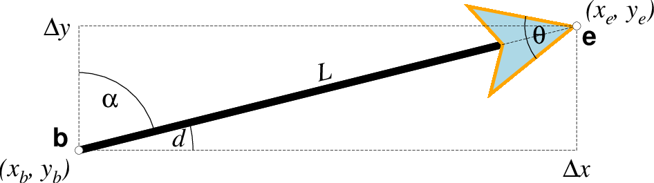
Vector attributes are controlled by options and modifiers. We will refer to this figure and the labels therein when introducing the corresponding modifiers. All vectors require you to specify the begin point \(x_b, y_b\) and the end point \(x_e, y_e\), or alternatively the direction d and length L, while for map projections we usually specify the azimuth \(\alpha\) instead.
Several modifiers may be appended to vector-producing options for specifying the placement of vector heads, their shapes, and the justification of the vector. Below, left and right refers to the side of the vector line when viewed from the beginning point (b) to the end point (e) of a line segment:
+aangle sets the angle \(\theta\) of the vector head apex [30].
+b places a vector head at the beginning of the vector path [none]. Optionally, append t for a terminal line, c for a circle, a for arrow [Default], i for tail, A for plain open arrow, and I for plain open tail. Further append l|r to only draw the left or right half-sides of this head [both sides].
+e places a vector head at the end of the vector path [none]. Optionally, append t for a terminal line, c for a circle, a for arrow [Default], i for tail, A for plain open arrow, and I for plain open tail. Further append l|r to only draw the left or right half-sides of this head [both sides].
+g[fill] sets the vector head fill [Default fill is used, which may be no fill]. Turn off vector head fill by not appending a fill. Some modules have a separate -Gfill option and if used will select the fill as well.
+hshape sets the shape of the vector head (range -2/2). Default is controlled by MAP_VECTOR_SHAPE [default is theme dependent]. A zero value produces no notch (e.g., the dashed line in the figure). Positive values moves the notch toward the head apex while a negative value moves away. The example above uses +h0.5.
+l draws half-arrows, using only the left side of specified heads [both sides].
+m places a vector head at the mid-point the vector path [none]. Append f or r for forward or reverse direction of the vector [forward]. Optionally, append t for a terminal line, c for a circle, a for arrow [Default], i for tail, A for plain open arrow, and I for plain open tail. Further append l|r to only draw the left or right half-sides of this head [both sides]. Cannot be combined with +b or +e.
+nnorm scales down vector attributes (pen thickness, head size) with decreasing length, where vector plot lengths shorter than norm will have their attributes scaled by length/norm [arrow attributes remains invariant to length]. For Cartesian vectors specify a length in plot units, while for geovectors specify a length in km.
+o[plon/plat] specifies the oblique pole for the great or small circles. Only needed for great circles if +q is given. If no pole is appended then we default to the north pole.
+p[pen] sets the vector pen attributes. If no pen is appended then the head outline is not drawn. [Default pen is half the width of stem pen, and head outline is drawn]. Above, we used +p2p,orange. The vector stem attributes are controlled by -W.
+q means the input direction, length data instead represent the start and stop opening angles of the arc segment relative to the given point. See +o to specify a specific pole for the arc [north pole].
+r draws half-arrows, using only the right side of specified heads [both sides].
+t[b|e]trim will shift the beginning or end point (or both) along the vector segment by the given trim; append suitable unit (c, i, or p). If the modifiers b|e are not used then trim may be two values separated by a slash, which is used to specify different trims for the beginning and end. Positive trims will shorted the vector while negative trims will lengthen it [no trim].
In addition, all but circular vectors may take these modifiers:
+jjust determines how the input x,y point relates to the vector. Choose from beginning [default], end, or center.
+s means the input angle, length are instead the \(x_e, y_e\) coordinates of the vector end point.
Finally, Cartesian vectors may take these modifiers:
+zscale expects input \(\Delta x, \Delta y\) vector components and uses the scale to convert to polar coordinates with length in given unit.
Note: Vectors were completely redesigned for GMT5 which separated the vector head (a polygon) from the vector stem (a line). In GMT4, the entire vector was a polygon and it could only be a straight Cartesian vector. Yes, the old GMT4 vector shape remains accessible if you specify a vector (-Sv|V) using the GMT4 syntax, explained here: size, if present, will be interpreted as \(t_w/h_l/h_w\) or tailwidth/headlength/halfheadwidth [Default is 0.075c/0.3c/0.25c (or 0.03i/0.12i/0.1i)]. By default, arrow attributes remain invariant to the length of the arrow. To have the size of the vector scale down with decreasing size, append +nnorm, where vectors shorter than norm will have their attributes scaled by length/norm. To center the vector on the balance point, use -Svb; to align point with the vector head, use -Svh; to align point with the vector tail, use -Svt [Default]. To give the head point’s coordinates instead of direction and length, use -Svs. Upper case B, H, T, S will draw a double-headed vector [Default is single head].
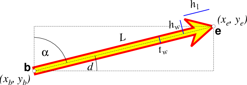
A GMT 4 vector has no separate pen for the stem -- it is all part of a Cartesian polygon. You may optionally fill and draw its outline. The modifiers listed above generally do not apply. Note: While the tailwidth (\(t_w\)) and headlength (\(h_l\)) parameters are given as indicated, the halfheadwidth (\(h_w\)) is oddly given as the half-width in GMT 4 so we retain that convention here (but have updated the documentation; blue lines indicate these three parameters).
Examples
Note: Below are some examples of valid syntax for this module.
The examples that use remote files (file names starting with @)
can be cut and pasted into your terminal for testing.
Other commands requiring input files are just dummy examples of the types
of uses that are common but cannot be run verbatim as written.
Note: Since many GMT plot examples are very short (i.e., one module call between the gmt begin and gmt end commands), we will often present them using the quick modern mode GMT Modern Mode One-line Commands syntax, which simplifies such short scripts.
To plot a half circle rose diagram of the data in the remote data file azimuth_lengths.txt (containing pairs of (azimuth, length in meters)), using a 5 degree bin sector width, on a circle of diameter = 10 cm, using a light blue shading, try:
gmt rose @azimuth_lengths.txt -: -A5 -JX10c -F -L -Glightblue -R0/1/0/180 -Bxaf+l"Fault length" -Byg30 -S -pdf half_rose
To plot a full circle wind rose diagram of the data in the file lines.r_az, on a circle of diameter = 10 cm, grid going out to radius = 500 units in steps of 100 with a 45 degree sector interval, using a solid pen (width = 0.5 point, and shown in landscape [Default] orientation with a timestamp and command line plotted, use:
gmt rose lines.az_r -R0/500/0/360 -JX10c -Bxg100 -Byg45 -B+t"Windrose diagram" -W0.5p -U+c -pdf rose
Redo the same plot but this time add orange vector heads to each direction (with nominal head size 0.5 cm but this will be reduced linearly for lengths less than 1 cm) and save the plot, use:
gmt rose lines.az_r -R0/500/0/360 -JX10c -Bxg100 -Byg45 -B+t"Windrose diagram" -M0.5c+e+gorange+n1c -W0.5p -U+c -pdf rose
Bugs
No default radial scale and grid settings for polar histograms. Users must run the module with -I to find max length in binned data set.
References
Berens, P., 2009, CircStat: A MATLAB Toolbox for Circular Statistics, J. Stat. Software, 31(10), 1-21.