(49) Analysis of the Atlantic seafloor depth/age relationship
In this example we show an example of data analysis using grids of seafloor depth and age for a region in the south Atlantic. We use module grdsample to convert the age grid to the same pixel registration used by the depth grid. Dumping separate x,y,z triplets with grd2xyz lets us paste the output back via gmtconvert to make binary tables of age,depth,depth. Here, depth is repeated in order to use blockmode for modal depth estimation and xyz2grd for mapping the data density. We image the density of (age,depth) points, overlay the modal depths and their robust uncertainty bars, and compute and plot two models for the expected depths as a function of age (see legend). Note we place most of the legend twice to achieve the thin-on-thick pen effect in the legend.
#!/bin/bash
#               GMT EXAMPLE 49
#               $Id$
#
# Purpose:      Illustrate data analysis using the seafloor depth/age relationship
# GMT modules:  blockmode, gmtmath, grdcontour, grdimage, grdsample, makecpt,
#		psbasemap, pslegend, psscale, psxy, xyz2grd
#

ps=example_49.ps

# Convert coarser age grid to pixel registration to match bathymetry grid
gmt grdsample age_gridline.nc -T -Gage_pixel.nc
# Image depths with color-coded age contours
gmt makecpt -Cabyss -T-7000/0 > depth.cpt
gmt grdimage depth_pixel.nc -Cdepth.cpt -JM6i -P -Baf -BWSne -X1.5i -K --FORMAT_GEO_MAP=dddF > $ps
gmt psxy -Rdepth_pixel.nc -J -O -K -W1p ridge.gmt >> $ps
gmt makecpt -Chot -T0/100/10 > age.cpt
gmt grdcontour age_pixel.nc -J -O -K -A+f14p -Cage.cpt -Wa0.1p+c -GL30W/22S/5E/13S >> $ps
gmt psscale -Rdepth_pixel.nc -J -DjTR+w2i/0.15i+h+o0.3i/0.15i -Cdepth.cpt -Baf+u" km" -W0.001 -F+p1p+gbeige -O -K >> $ps
# Obtain depth, age pairs by dumping grids and pasting results
gmt grd2xyz age_pixel.nc   -bof > age.bin
gmt grd2xyz depth_pixel.nc -bof > depth.bin
gmt convert -A age.bin depth.bin -bi3f -o2,5,5 -bo3f > depth-age.bin
# Create and map density grid of (age,depth) distribution
gmt xyz2grd -R0/100/-6500/0 -I0.25/25 -r depth-age.bin -bi3f -An -Gdensity.nc
gmt makecpt -Chot -T0/100 > density.cpt
gmt grdimage density.nc -JX6i/4i -Q -O -K -Cdensity.cpt -Y4.8i >> $ps
# Obtain modal depths every ~5 Myr
gmt blockmode -R0/100/-10000/0 -I5/10000 -r -E depth-age.bin -bi3f -o0,2,3 > modal.txt
# Compute Parsons & Sclater [1977] depth-age curve
# depth(t) =   350 * sqrt(t) + 2500, t < 70 Myr
#	   =  6400 - 3200 exp (-t/62.8), t > 70 Myr
gmt math -T0/100/0.1 T SQRT 350 MUL 2500 ADD T 70 LE MUL 6400 T 62.8 DIV NEG EXP 3200 MUL SUB T 70 GT MUL ADD NEG = ps.txt
gmt psxy -Rdensity.nc -J -O -K ps.txt -W4p,green >> $ps
gmt psxy -R -J -O -K ps.txt -W1p >> $ps
# Compute Stein & Stein [1992] depth-age curve
# depth(t) =  365 * sqrt(t) + 2600,  t < 20 Myr
#	   = 5651 - 2473 * exp (-0.0278*t), t > 20 Myr
gmt math -T0/100/0.1 T SQRT 365 MUL 2600 ADD T 20 LE MUL 5651 T -0.0278 MUL EXP 2473 MUL SUB T 20 GT MUL ADD NEG = ss.txt
# Plot curves and place the legend
gmt psxy -R -J -O -K ss.txt -W4p,white  >> $ps
gmt psxy -R -J -O -K ss.txt -W1p >> $ps
gmt psxy -R -J -Ss0.4c -O -K -Gblue modal.txt -Ey+p1p,blue >> $ps
gmt psxy -R -J -Ss0.1c -O -K -Gwhite modal.txt >> $ps
gmt psbasemap -R0/100/0/6.5 -JX6i/-4i -Bxaf+u" Myr" -Byaf+u" km" -BWsNe -O -K >> $ps
gmt pslegend -R -J -O -K -DjRT+w2.5i+o0.1i -F+p1p+gbeige+s << EOF >> $ps
S 0.2i - 0.35i - 4p,green 0.5i Parsons & Sclater (1977)
S 0.2i - 0.35i - 4p,white 0.5i Stein & Stein (1992)
S 0.2i s 0.15i blue - 0.5i Modal depth estimates
EOF
gmt pslegend -R -J -O -K -DjRT+w2.5i+o0.1i << EOF >> $ps
S 0.2i - 0.35i - 1p 0.3i
S 0.2i - 0.35i - 1p 0.3i
S 0.2i s 0.1c white - 0.3i
EOF
gmt psxy -R -J -O -T >> $ps
rm -f age_pixel.nc age.bin depth.bin depth-age.bin density.nc modal.txt ps.txt ss.txt *.cpt
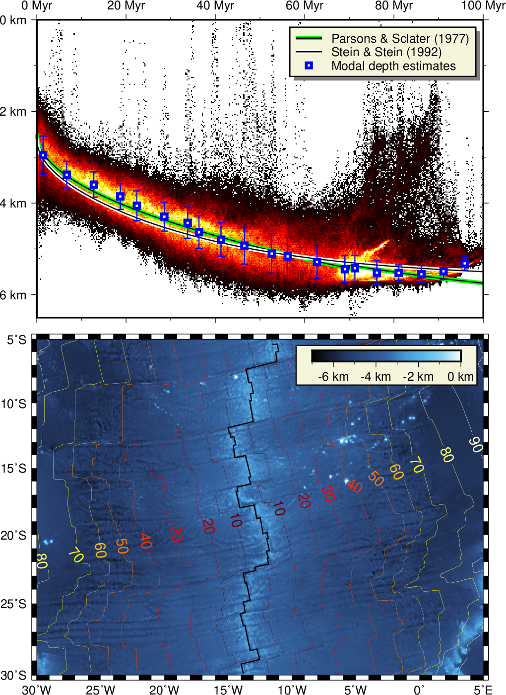
Seafloor depth vs. age in the south Atlantic.