math will perform operations like add, subtract, multiply, and
numerous other operands on one or more table data files or constants using
Reverse Polish Notation (RPN)
syntax. Arbitrarily complicated expressions may therefore be evaluated; the
final result is written to an output file [or standard output]. Data
operations are element-by-element, not matrix manipulations (except
where noted). Some operators only require one operand (see below). If no
data tables are used in the expression then options -T, -N can
be set (and optionally -bo to indicate the
data type for binary tables). If STDIN is given, the standard input will
be read and placed on the stack as if a file with that content had been
given on the command line. By default, all columns except the “time”
column are operated on, but this can be changed (see -C).
Complicated or frequently occurring expressions may be coded as a macro
for future use or stored and recalled via named memory locations.
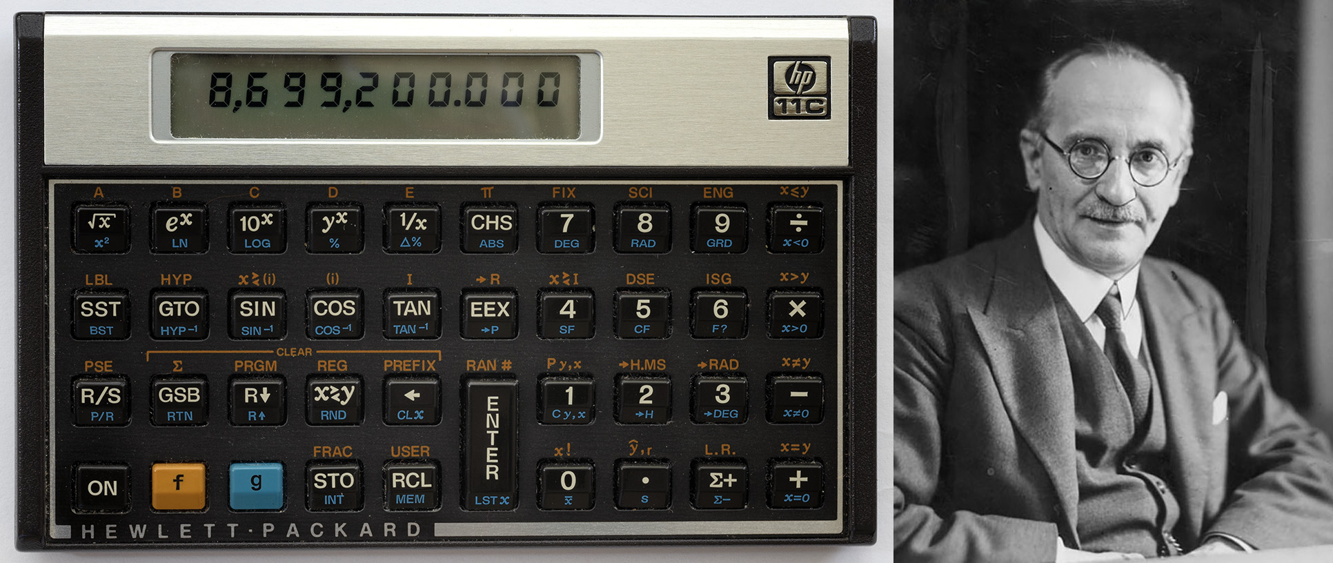
Hewlett-Packard made lots of calculators (left) using Reverse Polish Notation,
which is a post-fix system for mathematical notion originally developed by
Jan_Łukasiewicz (right).
Here, operands are entered first followed by an operator, e.g., “3 5 +” instead
of “3 + 5 =” (photo courtesy of John W. Robbins).
If operand can be opened as a file it will be read as an ASCII (or
binary, see -bi) table data file. If not
a file, it is interpreted as a numerical constant or a special
symbol (see below). The special argument STDIN means that standard input
will be read and placed on the stack; STDIN can appear more than
once if necessary.
outfile
The name of a table data file that will hold the final result. If
not given then the output is sent to standard output.
Requires -N and will partially initialize a table with values
from the given file t_f(t) containing t and f(t) only. The t is
placed in column t_col while f(t) goes into column n_col - 1
(see -N) and is called b. The stack table is then the \(m \times (n+1)\)
augmented matrix [ A | b ] and you want to solve for the least squares solution
x to the matrix equation Ax = b. Usually, you will need
to fill in the remaining columns in A using the various functions
that defines the linear model you are trying to fit. If used with operators
LSQFIT and SVDFIT you can optionally append some modifiers:
+e - Evaluate the solution and write a data set with four columns:
t, f(t), the model solution and residuals at t, respectively
[Default writes one column with model coefficients x].
+r - Only place f(t) (i.e., b) and leave the A part of the
augmented matrix equation alone.
+s - Your t_f(t) has a third column with 1-sigma uncertainties, or
+w - Your t_f(t table has a third column with weights.
Note: If either +s or +w are used we find the weighted solution. The weights
(or sigmas) will be output as the last column if +e is in effect.
-Ccols
Select the columns that will be operated on until next occurrence of
-C. List columns separated by commas; ranges like 1,3-5,7 are
allowed, plus -Cx can be used for -C0 and -Cy can be used for -C1.
-C (no arguments) resets the default action of using
all columns except time column (see -N). -Ca selects all
columns, including time column, while -Cr reverses (toggles) the
current choices. When -C is in effect it also controls which
columns from a file will be placed on the stack.
-Eeigen
Sets the minimum eigenvalue used by operators LSQFIT and SVDFIT [1e-7].
Smaller eigenvalues are set to zero and will not be considered in the
solution.
-I
Reverses the output row sequence from ascending time to descending [ascending].
-Nn_col[/t_col]
Select the number of columns and optionally the column number that
contains the “time” variable [0]. Columns are numbered starting at 0
[2/0]. If input files are specified then -N will add any missing
columns.
-Q[c|i|p|n]
Quick mode for scalar calculation. Internally sets the equivalent of -Ca-N1/0 -T1.
In this mode, constants may have dimensional units (i.e., c, i, or p),
and will be converted to internal inches before computing. If one or more constants
with units are encountered then the final answer will be reported in the unit set by
PROJ_LENGTH_UNIT, unless overridden by appending another unit. Alternatively,
append n for a non-dimensional result, meaning no unit conversion during output.
To avoid any unit conversion on input, just do not use units.
-S[f|l]
Only report the first or last row of the results [Default outputs all
rows]. This is useful if you have computed a statistic (say the
MODE) and only want to report a single number instead of
numerous records with identical values. Append l to get the last
row and f to get the first row only [Default].
-T[min/max/inc[+b|i|l|n]|file|list]
Required when no input files are given. Builds an array for
the “time” column (see -N). If there is no time column
(i.e., your input has only data columns), give -T with
no arguments; this also implies -Ca.
For details on array creation, see Generate 1-D Array.
We will demonstrate the use of options for creating 1-D arrays via gmtmath.
Make an evenly spaced coordinate array from min to max in steps of inc, e.g.:
Append +b if we should take \(\log_2\) of min and max, get their nearest integers,
build an equidistant \(\log_2\)-array using inc integer increments in \(\log_2\), then undo
the \(\log_2\) conversion. E.g., -T3/20/1+b will produce this sequence:
gmtmath-o0-T3/20/1+bT=4816
Append +l if we should take \(\log_{10}\) of min and max and build an
array where inc can be 1 (every magnitude), 2, (1, 2, 5 times magnitude) or 3
(1-9 times magnitude). E.g., -T7/135/2+l will produce this sequence:
gmtmath-o0-T7/135/2+lT=102050100
For output values less frequently than every magnitude, use a negative integer inc:
gmtmath-o0-T1e-4/1e4/-2+lT=0.0001
0.01
110010000
Append +i if inc is a fractional number and it is cleaner to give its reciprocal
value instead. To set up times for a 24-frames per second animation lasting 1 minute, run:
Alternatively, let inc be a file with output coordinates in the first column,
or provide a comma-separated list of specific coordinates, such as the first 6
Fibonacci numbers:
gmtmath-o0-T0,1,1,2,3,5T=011235
Notes: (1) If you need to pass the list nodes via a dataset file yet be understood
as a list (i.e., no interpolation), then you must set the file header to contain the string “LIST”. (2) Should
you need to ensure that the coordinates are unique and sorted (in case the
file or list are not sorted or have duplicates) then supply the +u modifier.
If you only want a single value
then you must append a comma to distinguish the list from the setting of an increment.
If the module allows you to set up an absolute time series, append a valid time unit from the list
year, month, day, hour, minute, and second
to the given increment; add +t to ensure time column (or use -f). Note: The internal time
unit is still controlled independently by TIME_UNIT. The first 7 days of March 2020:
A few modules allow for +a which will paste the coordinate array to the output table.
Likewise, if the module allows you to set up a spatial distance series (with distances computed
from the first two data columns), specify a new increment as inc with a geospatial distance unit from the list
degree (arc), minute (arc), second (arc), meter, foot, kilometer,
Miles (statute), nautical miles, or survey foot; see -j for calculation mode.
To interpolate Cartesian distances instead, you must use the special unit c.
Finally, if you are only providing an increment and will obtain min and max from the data, then it is
possible (max - min)/inc is not an integer, as required. If so, then inc will be adjusted to fit the range.
Alternatively, append +e to keep inc exact and adjust max instead (keeping min fixed).
The ASCII output formats of numerical data are controlled by parameters
in your gmt.conf file. Longitude and latitude are formatted
according to FORMAT_GEO_OUT, absolute time is
under the control of FORMAT_DATE_OUT and
FORMAT_CLOCK_OUT, whereas general floating point values are formatted
according to FORMAT_FLOAT_OUT. Be aware that the format in effect
can lead to loss of precision in ASCII output, which can lead to various
problems downstream. If you find the output is not written with enough
precision, consider switching to binary output (-bo if available) or
specify more decimals using the FORMAT_FLOAT_OUT setting.
The operators PLM and PLMg calculate the associated Legendre
polynomial of degree L and order M in x which must satisfy \(-1 \leq x \leq +1\)
and \(0 \leq M \leq L\). Here, x, L, and M are the three arguments preceding the
operator. PLM is not normalized and includes the Condon-Shortley
phase \((-1)^M\). PLMg is normalized in the way that is most commonly
used in geophysics. The Condon-Shortley phase can be added by using -M as argument.
PLM will overflow at higher degrees, whereas PLMg is stable
until ultra high degrees (at least 3000).
Files that have the same names as some operators, e.g., ADD,
SIGN, =, etc. should be identified by prepending the current
directory (i.e., ./).
The stack depth limit is hard-wired to 100.
All functions expecting a positive radius (e.g., LOG, KEI,
etc.) are passed the absolute value of their argument.
The DDT and D2DT2 functions only work on regularly spaced data.
All derivatives are based on central finite differences, with
natural boundary conditions.
ROOTS must be the last operator on the stack, only followed by =.
You may store intermediate calculations to a named variable that you may
recall and place on the stack at a later time. This is useful if you
need access to a computed quantity many times in your expression as it
will shorten the overall expression and improve readability. To save a
result you use the special operator STO@label, where label
is the name you choose to give the quantity. To recall the stored result
to the stack at a later time, use [RCL]@label, i.e., RCL
is optional. To clear memory you may use CLR@label. Note that
both STO and CLR leave the stack unchanged.
The bitwise operators
(BITAND, BITLEFT, BITNOT, BITOR, BITRIGHT,
BITTEST, and BITXOR) convert a tables’s double precision values
to unsigned 64-bit ints to perform the bitwise operations. Consequently,
the largest whole integer value that can be stored in a double precision
value is 253 or 9,007,199,254,740,992. Any higher result will be masked
to fit in the lower 54 bits. Thus, bit operations are effectively limited
to 54 bits. All bitwise operators return NaN if given NaN arguments or
bit-settings <= 0.
TAPER will interpret its argument to be a width in the same units as
the time-axis, but if no time is provided (i.e., plain data tables) then
the width is taken to be given in number of rows.
The color-triplet conversion functions (RGB2HSV, etc.) includes not
only r,g,b and h,s,v triplet conversions, but also l,a,b (CIE L a b ) and
sRGB (x,y,z) conversions between all four color spaces. These functions
behave differently whether -Q is used or not. With -Q we expect
three input constants and we place three output results on the stack. Since
only the top stack item is printed, you must use operators such as POP and
ROLL to get to the item of interest. Without -Q, these operators work
across the three columns and modify the three column entries, returning their
result as a single three-column item on the stack.
Users may save their favorite operator combinations as macros via the
file gmtmath.macros in their current or user directory. The file may contain
any number of macros (one per record); comment lines starting with # are
skipped. The format for the macros is name = arg1 arg2 … arg2
[ : comment] where name is how the macro will be used. When this
operator appears on the command line we simply replace it with the
listed argument list. No macro may call another macro. As an example,
the following macro expects that the time-column contains seafloor ages
in Myr and computes the predicted half-space bathymetry:
DEPTH = SQRT 350 MUL 2500 ADD NEG : usage: DEPTH to return
half-space seafloor depths
Note: Because geographic or time constants may be present in a macro, it
is required that the optional comment flag (:) must be followed by a space.
As another example, we show a macro GPSWEEK which determines which GPS week
a timestamp belongs to:
GPSWEEK = 1980-01-06T00:00:00 SUB 86400 DIV 7 DIV FLOOR : usage: GPS week without rollover
When -Ccols is set then any operation, including loading of data from files, will
restrict which columns are affected.
To avoid unexpected results, note that if you issue a -Ccols option before you load
in the data then only those columns will be updated, hence the unspecified columns will be zero.
On the other hand, if you load the file first and then issue -Ccols then the unspecified
columns will have been loaded but are then ignored until you undo the effect of -C.
If input data have more than one column and the “time” column (set via -N [0])
contains absolute time, then the default output format for any other columns containing
absolute time will be reset to relative time. Likewise, in scalar mode (-Q) the
time column will be operated on and hence it also will be formatted as relative
time. Finally, if -C is used to include “time” in the columns operated on then
we likewise will reset that column’s format to relative time. The user can override this behavior with a
suitable -f or -fo setting. Note: We cannot guess what your operations on the
time column will do, hence this default behavior. As examples, if you are computing time differences
then clearly relative time formatting is required, while if you are computing new absolute times
by, say, adding an interval to absolute times then you will need to use -fo to set
the output format for such columns to absolute time.
If you use -Q to do simple calculations, please note that the support for dimensional units is
limited to converting a number ending in c, i, or p to internal inches. Thus, while you can run
“gmt -Qc 1c 1c MUL =”, you may be surprised that the output area is not 1 cm squared. The reason is
that gmt math cannot keep track of what unit any particular item on the stack might be so it will
assume it is internally in inches and then scale the final output to cm. In this particular case,
the unit is in inches squared and scaling by 2.54 once will give 0.3937 inch times cm as the unit.
Thus, conversions only work for linear unit calculations, such as gmt math -Qp 1c 0.5i ADD =, which
will return the result as 64.34 points.
Note: Below are some examples of valid syntax for this module.
The examples that use remote files (file names starting with @)
can be cut and pasted into your terminal for testing.
Other commands requiring input files are just dummy examples of the types
of uses that are common but cannot be run verbatim as written.
To add two plot dimensions of different units, we can run
length=$(gmtmath-Q15c2iSUB=)
To compute the ratio of two plot dimensions of different units, we select non-dimensional output and run
ratio=$(gmtmath-Qn15c2iDIV=)
To take the square root of the content of the second data column being
piped through gmtmath by process1 and pipe it through a 3rd process, use
process1|gmtmathSTDINSQRT=|process3
To take \(\log_{10}\) of the average of 2 data files, use
gmtmathfile1.txtfile2.txtADD0.5MULLOG10=file3.txt
Given the file samples.txt, which holds seafloor ages in m.y. and seafloor
depth in m, use the relation depth(in m) = 2500 + 350 * sqrt (age) to
print the depth anomalies:
gmtmathsamples.txtTSQRT350MUL2500ADDSUB=|lpr
To take the average of columns 1 and 4-6 in the three data sets sizes.1,
sizes.2, and sizes.3, use
To take the 1-column data set ages.txt and calculate the modal value and
assign it to a variable, try
mode_age=$(gmtmath-S-Tages.txtMODE=)
To evaluate the dilog(x) function for coordinates given in the file t.txt:
gmtmath-Tt.txtTDILOG=dilog.txt
To demonstrate the use of stored variables, consider this sum of the
first 3 cosine harmonics where we store and repeatedly recall the
trigonometric argument (2*pi*T/360):
To use gmtmath as a RPN Hewlett-Packard calculator on scalars (i.e., no
input files) and calculate arbitrary expressions, use the -Q option.
As an example, we will calculate the value of Kei (((1 + 1.75)/2.2) +
cos (60)) and store the result in the shell variable z:
z=$(gmtmath-Q11.75ADD2.2DIV60COSDADDKEI=)
To convert the r,g,b value for yellow to h,s,v and save the hue, try
hue=$(gmtmath-Q2552550RGB2HSVPOPPOP=)
To use gmtmath as a general least squares equation solver, imagine
that the current table is the augmented matrix [ A | b ] and you want
the least squares solution x to the matrix equation A * x = b. The
operator LSQFIT does this; it is your job to populate the matrix
correctly first. The -A option will facilitate this. Suppose you
have a 2-column file ty.txt with t and y and you would like to fit
a the model y(t) = a + b*t + c*H(t-t0), where H(t) is the Heaviside step
function for a given t0 = 1.55. Then, you need a 4-column augmented
table loaded with t in column 1 and your observed y in column 3. The
calculation becomes
Note we use the -C option to select which columns we are working on,
then make active all the columns we need (here all of them, with
-Ca) before calling LSQFIT. The second and fourth columns (col
numbers 1 and 3) are preloaded with t and y, respectively, the other
columns are zero. If you already have a pre-calculated table with the
augmented matrix [ A | b ] in a file (say lsqsys.txt), the least squares
solution is simply
gmtmath-Tlsqsys.txtLSQFIT=solution.txt
Users must be aware that when -C controls which columns are to be
active the control extends to placing columns from files as well.
Contrast the different result obtained by these very similar commands:
echo1234|gmtmathSTDIN-C31ADD=1235
versus
echo1234|gmtmath-C3STDIN1ADD=0005
To calculate how many days there were in the 80s decade:
gmtmath-Q1991-01-01T1981-01-01TSUB--TIME_UNIT=d=
To determine the 1000th day since the beginning of the millennium:
Abramowitz, M., and I. A. Stegun, 1964, Handbook of Mathematical
Functions, Applied Mathematics Series, vol. 55, Dover, New York.
Holmes, S. A., and W. E. Featherstone, 2002, A unified approach to the
Clenshaw summation and the recursive computation of very high degree and
order normalized associated Legendre functions. Journal of Geodesy,
76, 279-299.
Press, W. H., S. A. Teukolsky, W. T. Vetterling, and B. P. Flannery,
1992, Numerical Recipes, 2nd edition, Cambridge Univ., New York.
Spanier, J., and K. B. Oldman, 1987, An Atlas of Functions, Hemisphere
Publishing Corp.
More on Reverse Polish Notation
Reverse Polish Notation (RPN) or postfix notation is widely used in computer science because of the simplicity of implementing a
stack-based computation system. The PostScipt language we used to make GMT graphics is postfix, for instance.
To learn more about RPN or postfix, watch this YouTube video explanation: