nearneighbor
Grid table data using a "Nearest neighbor" algorithm
Synopsis
gmt nearneighbor [ table ] -Goutgrid -Iincrement -Rregion -Ssearch_radius [ -Eempty ] [-Nsectors[+mmin_sectors]|n] [ -V[level] ] [ -W ] [ -aflags ] [ -bibinary ] [ -di[+ccol]nodata ] [ -eregexp ] [ -fflags ] [ -hheaders ] [ -iflags ] [ -nflags ] [ -qiflags ] [ -rreg ] [ -wflags ] [ -:[i|o] ] [ --PAR=value ]
Note: No space is allowed between the option flag and the associated arguments.
Description
nearneighbor reads arbitrarily located (x,y,z[,w]) triples [quadruplets] from standard input [or table] and uses a nearest neighbor algorithm to assign a weighted average value to each node that has one or more data points within a search radius (R) centered on the node with adequate coverage across a subset of the chosen sectors. The node value is computed as a weighted mean of the nearest point from each sector inside the search radius. The weighting function and the averaging used is given by
where n is the number of data points that satisfy the selection criteria and \(r_i\) is the distance from the node to the i’th data point. If no data weights are supplied then \(w_i = 1\).
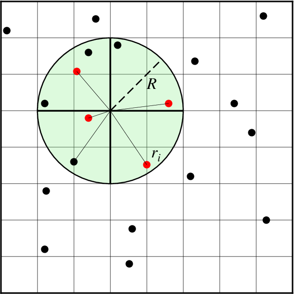
Search geometry includes the search radius (R) which limits the points considered and the number of sectors (here 4), which restricts how points inside the search radius contribute to the value at the node. Only the closest point in each sector (red circles) contribute to the weighted estimate.
Required Arguments
- table
3 [or 4, see -W] column ASCII file(s) [or binary, see -bi] holding (x,y,z[,w]) data values. If no file is specified, nearneighbor will read from standard input.
-Goutgrid[=ID][+ddivisor][+ninvalid] [+ooffset|a][+sscale|a] [:driver[dataType][+coptions]]
Give the name of the output grid file. Optionally, append =ID for writing a specific file format (See full description). The following modifiers are supported:
+d - Divide data values by given divisor [Default is 1].
+n - Replace data values matching invalid with a NaN.
+o - Offset data values by the given offset, or append a for automatic range offset to preserve precision for integer grids [Default is 0].
+s - Scale data values by the given scale, or append a for automatic scaling to preserve precision for integer grids [Default is 1].
Note: Any offset is added before any scaling. +sa also sets +oa (unless overridden). To write specific formats via GDAL, use = gd and supply driver (and optionally dataType) and/or one or more concatenated GDAL -co options using +c. See the “Writing grids and images” cookbook section for more details.
- -Ix_inc[+e|n][/y_inc[+e|n]]
Set the grid spacing as x_inc [and optionally y_inc].
Geographical (degrees) coordinates: Optionally, append an increment unit. Choose among:
m to indicate arc minutes
s to indicate arc seconds
e (meter), f (foot), k (km), M (mile), n (nautical mile) or u (US survey foot), in which case the increment will be converted to the equivalent degrees longitude at the middle latitude of the region (the conversion depends on PROJ_ELLIPSOID). If y_inc is given but set to 0 it will be reset equal to x_inc; otherwise it will be converted to degrees latitude.
All coordinates: The following modifiers are supported:
+e to slightly adjust the max x (east) or y (north) to fit exactly the given increment if needed [Default is to slightly adjust the increment to fit the given domain].
+n to define the number of nodes rather than the increment, in which case the increment is recalculated from the number of nodes, the registration (see GMT File Formats), and the domain. Note: If -Rgrdfile is used then the grid spacing and the registration have already been initialized; use -I and -R to override these values.
- -Rxmin/xmax/ymin/ymax[+r][+uunit]
Specify the region of interest. (See full description) (See cookbook information).
- -Ssearch_radius
Sets the search_radius that determines which data points are considered close to a node. Append the distance unit (see Units).
Optional Arguments
- -Eempty
Set the value assigned to empty nodes [NaN].
- -V[level]
Select verbosity level [w]. (See full description) (See cookbook information).
- -Nsectors[+mmin_sectors]|n
The circular search area centered on each node is divided into sectors sectors. Average values will only be computed if there is at least one value inside each of at least min_sectors of the sectors for a given node. Nodes that fail this test are assigned the value NaN (but see -E). If +m is omitted then min_sectors is set to be at least 50% of sectors (i.e., rounded up to next integer) [Default is a quadrant search with 100% coverage, i.e., sectors = min_sectors = 4]. Note that only the nearest value per sector enters into the averaging; the more distant points are ignored. Alternatively, use -Nn to call GDALʻs nearest neighbor algorithm instead.
- -W
Input data have a 4th column containing observation point weights. These are multiplied with the geometrical weight factor to determine the actual weights used in the calculations.
- -a[[col=]name[,…]] (more …)
Set aspatial column associations col=name.
- -birecord[+b|l] (more …)
Select native binary format for primary table input. [Default is 3 (or 4 if -W is set) columns].
- -dinodata[+ccol] (more …)
Replace input columns that equal nodata with NaN.
- -e[~]“pattern” | -e[~]/regexp/[i] (more …)
Only accept data records that match the given pattern.
- -f[i|o]colinfo (more …)
Specify data types of input and/or output columns.
- -gx|y|z|d|X|Y|Dgap[u][+a][+ccol][+n|p] (more …)
Determine data gaps and line breaks.
- -h[i|o][n][+c][+d][+msegheader][+rremark][+ttitle] (more …)
Skip or produce header record(s).
- -icols[+l][+ddivisor][+sscale|d|k][+ooffset][,…][,t[word]] (more …)
Select input columns and transformations (0 is first column, t is trailing text, append word to read one word only).
- -n[b|c|l|n][+a][+bBC][+tthreshold]
Append +bBC to set any boundary conditions to be used, adding g for geographic, p for periodic, or n for natural boundary conditions. For the latter two you may append x or y to specify just one direction, otherwise both are assumed. [Default is geographic if grid is geographic].
- -qi[~]rows|limits[+ccol][+a|f|s] (more …)
Select input rows or data limit(s) [default is all rows].
- -r[g|p] (more …)
Set node registration [gridline].
- -wy|a|w|d|h|m|s|cperiod[/phase][+ccol] (more …)
Convert an input coordinate to a cyclical coordinate.
- -:[i|o] (more …)
Swap 1st and 2nd column on input and/or output.
- -^ or just -
Print a short message about the syntax of the command, then exit (NOTE: on Windows just use -).
- -+ or just +
Print an extensive usage (help) message, including the explanation of any module-specific option (but not the GMT common options), then exit.
- -? or no arguments
Print a complete usage (help) message, including the explanation of all options, then exit.
- --PAR=value
Temporarily override a GMT default setting; repeatable. See gmt.conf for parameters.
Units
For map distance unit, append unit d for arc degree, m for arc minute, and s for arc second, or e for meter [Default], f for foot, k for km, M for statute mile, n for nautical mile, and u for US survey foot. By default we compute such distances using a spherical approximation with great circles (-jg) using the authalic radius (see PROJ_MEAN_RADIUS). You can use -jf to perform “Flat Earth” calculations (quicker but less accurate) or -je to perform exact geodesic calculations (slower but more accurate; see PROJ_GEODESIC for method used).
Grid Values Precision
Regardless of the precision of the input data, GMT programs that create grid files will internally hold the grids in 4-byte floating point arrays. This is done to conserve memory and furthermore most if not all real data can be stored using 4-byte floating point values. Data with higher precision (i.e., double precision values) will lose that precision once GMT operates on the grid or writes out new grids. To limit loss of precision when processing data you should always consider normalizing the data prior to processing.
Examples
Note: Below are some examples of valid syntax for this module.
The examples that use remote files (file names starting with @)
can be cut and pasted into your terminal for testing.
Other commands requiring input files are just dummy examples of the types
of uses that are common but cannot be run verbatim as written.
To grid the data in the remote file @ship_15.txt at 5x5 arc minutes using a search radius of 15 arch minutes, and plot the resulting grid using default projection and colors, try:
gmt begin map
  gmt nearneighbor @ship_15.txt -R245/255/20/30 -I5m -Ggrid.nc -S15m
  gmt grdimage grid.nc -B
gmt end show
To create a gridded data set from the file seaMARCII_bathy.lon_lat_z using a 0.5 min grid, a 5 km search radius, using an octant search with 100% sector coverage, and set empty nodes to -9999:
gmt nearneighbor seaMARCII_bathy.lon_lat_z -R242/244/-22/-20 -I0.5m -E-9999 -Gbathymetry.nc -S5k -N8+m8
To make a global grid file from the data in geoid.xyz using a 1 degree grid, a 200 km search radius, spherical distances, using an quadrant search, and set nodes to NaN only when fewer than two quadrants contain at least one value:
gmt nearneighbor geoid.xyz -R0/360/-90/90 -I1 -Lg -Ggeoid.nc -S200k -N4
See Also
blockmean, blockmedian, blockmode, gmt, greenspline, sphtriangulate, surface, triangulate