grdmath

Reverse Polish Notation (RPN) calculator for grids (element by element)

Synopsis

gmt grdmath [ -Amin_area[/min_level/max_level][+a[g|i][s|S]][+l|r][+ppercent] ] [ -C[cpt] ] [ -Dresolution[+f] ] [ -Iincrement ] [ -M ] [ -N ] [ -Rregion ] [ -S ] [ -V[level] ] [ -aflags ] [ -bibinary ] [ -dinodata[+ccol] ] [ -eregexp ] [ -fflags ] [ -ggaps ] [ -hheaders ] [ -iflags ] [ -nflags ] [ -rreg ] [ -x[[-]n] ] [ --PAR=value ] operand [ operand ] OPERATOR [ operand ] OPERATOR= outgrid

Note: No space is allowed between the option flag and the associated arguments.

Description

grdmath will perform operations like add, subtract, multiply, and hundreds of other operands on one or more grid files or constants using Reverse Polish Notation (RPN) syntax. Arbitrarily complicated expressions may therefore be evaluated; the final result is written to an output grid file. Grid operations are element-by-element, not matrix manipulations. Some operators only require one operand (see below). If no grid files are used in the expression then options -R, -I must be set (and optionally -rreg). The expression = outgrid can occur as many times as the depth of the stack allows in order to save intermediate results. Complicated or frequently occurring expressions may be coded as a macro for future use or stored and recalled via named memory locations.

_images/RPN_fig.jpg

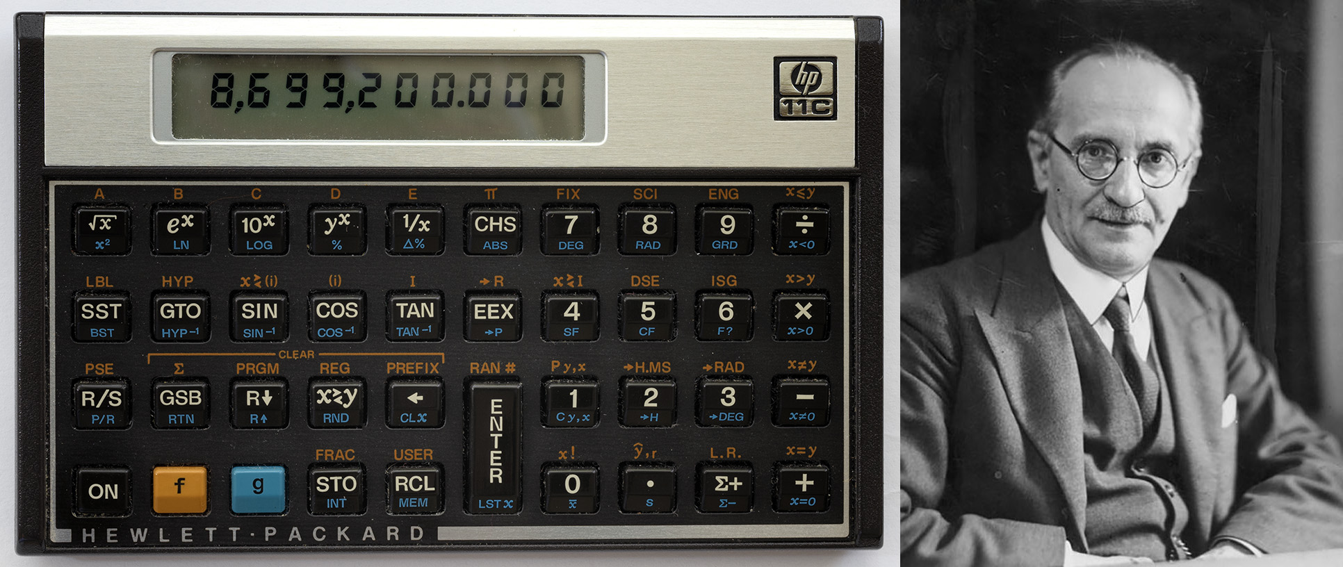
Hewlett-Packard made lots of calculators (left) using Reverse Polish Notation, which is a post-fix system for mathematical notion originally developed by Jan_Łukasiewicz (right). Here, operands are entered first followed by an operator, e.g., “3 5 +” instead of “3 + 5 =” (photo courtesy of John W. Robbins).

Required Arguments

operand

If operand can be opened as a file it will be read as a grid file. If not a file, it is interpreted as a numerical constant or a special symbol (see below).

outgrid

The name of a 2-D grid file that will hold the final result. (See Grid File Formats).

Optional Arguments

-Amin_area[/min_level/max_level][+a[g|i][s|S]][+l|r][+ppercent]

Features with an area smaller than min_area in km2 or of hierarchical level that is lower than min_level or higher than max_level will not be plotted [Default is 0/0/4 (all features)]. Level 2 (lakes) contains regular lakes and wide river bodies which we normally include as lakes. Several modifiers provide further control:

  • +a - Control special aspects of the Antarctica coastline. Append one of g|s|s|S:

    • g - Selects the Antarctica ice grounding line as the coastline.

    • i - Selects the ice shelf boundary as the coastline for Antarctica [Default].

    • s - Skip all GSHHG features below 60S (For users who wish to utilize their own Antarctica (with islands) coastline).

    • S - Like s but skip instead all features north of 60S.

  • +l - Only regular lakes and exclude river-lakes.

  • +p - Append percent to exclude polygons whose percentage area of the corresponding full-resolution feature is less than percent.

  • +r - Only select river-lakes and exclude regular lakes.

See GSHHG Information below for more details. (-A is only relevant to the LDISTG operator)

-C[cpt]

Retain the grid’s default CPT (if it has one), or alternatively replace it with a new default cpt [Default removes any default CPT from the output grid].

-Dresolution[+f]

Selects the resolution of the data set to use with the operator LDISTG ((f)ull, (h)igh, (i)ntermediate, (l)ow, and (c)rude). The resolution drops off by 80% between data sets [Default is l]. Append +f to automatically select a lower resolution should the one requested not be available [abort if not found].

-Ix_inc[+e|n][/y_inc[+e|n]]

Set the grid spacing as x_inc [and optionally y_inc].

Geographical (degrees) coordinates: Optionally, append an increment unit. Choose among:

  • d - Indicate arc degrees

  • m - Indicate arc minutes

  • s - Indicate arc seconds

If one of e (meter), f (foot), k (km), M (mile), n (nautical mile) or u (US survey foot), the the increment will be converted to the equivalent degrees longitude at the middle latitude of the region (the conversion depends on PROJ_ELLIPSOID). If y_inc is not given or given but set to 0 it will be reset equal to x_inc; otherwise it will be converted to degrees latitude.

All coordinates: The following modifiers are supported:

  • +e - Slightly adjust the max x (east) or y (north) to fit exactly the given increment if needed [Default is to slightly adjust the increment to fit the given domain].

  • +n - Define the number of nodes rather than the increment, in which case the increment is recalculated from the number of nodes, the registration (see GMT File Formats), and the domain. Note: If -Rgrdfile is used then the grid spacing and the registration have already been initialized; use -I and -R to override these values.

-M

By default any derivatives calculated are in z_units/x(or y)_units. However, the user may choose this option to convert dx,dy in degrees of longitude,latitude into meters using a flat Earth approximation, so that gradients are in z_units/meter.

-N

Turn off strict domain match checking when multiple grids are manipulated [Default will insist that each grid domain is within \(10^{-4}\) times the grid spacing of the domain of the first grid listed].

-Rxmin/xmax/ymin/ymax[+r][+uunit]

Specify the region of interest. (See full description) (See cookbook information).

-S

Reduce (i.e., collapse) the entire stack to a single grid by applying the next operator to all co-registered nodes across the entire stack. You must specify -S after listing all of your grids. Note: You can only follow -S with a reducing operator, i.e., from the list ADD, AND, MAD, LMSSCL, MAX, MEAN, MEDIAN, MIN, MODE, MUL, RMS, STD, SUB, VAR or XOR.

-V[level]

Select verbosity level [w]. (See full description) (See cookbook information).

-a[[col=]name[,]] (more …)

Set aspatial column associations col=name.

-birecord[+b|l] (more …)

Select native binary format for primary table input. The binary input option only applies to the data files needed by operators LDIST, PDIST, and INSIDE.

-dinodata[+ccol] (more …)

Replace input columns that equal nodata with NaN.

-e[~]“pattern” | -e[~]/regexp/[i] (more …)

Only accept data records that match the given pattern.

-f[i|o]colinfo (more …)

Specify data types of input and/or output columns.

-gx|y|z|d|X|Y|Dgap[u][+a][+ccol][+n|p] (more …)

Determine data gaps and line breaks.

-h[i|o][n][+c][+d][+msegheader][+rremark][+ttitle] (more …)

Skip or produce header record(s).

-icols[+l][+ddivisor][+sscale|d|k][+ooffset][,][,t[word]] (more …)

Select input columns and transformations (0 is first column, t is trailing text, append word to read one word only).

-n[b|c|l|n][+a][+bBC][+c][+tthreshold] (more …)

Select interpolation mode for grids.

-r[g|p] (more …)

Set node registration [gridline]. Only used with -R -I.

-x[[-]n] (more …)

Limit number of cores used in multi-threaded algorithms (OpenMP required).

-^ or just -

Print a short message about the syntax of the command, then exit (Note: on Windows just use -).

-+ or just +

Print an extensive usage (help) message, including the explanation of any module-specific option (but not the GMT common options), then exit.

-? or no arguments

Print a complete usage (help) message, including the explanation of all options, then exit.

--PAR=value

Temporarily override a GMT default setting; repeatable. See gmt.conf for parameters.

Operators

Choose among the following operators. “Args” are the number of input and output arguments.

Operator

Args

Returns

Type of function

ABS

1 1

Absolute value of A

Arithmetic

ACOS

1 1

Inverse cosine (result in radians)

Calculus

ACOSD

1 1

Inverse cosine (result in degrees)

Calculus

ACOSH

1 1

Inverse hyperbolic cosine

Calculus

ACOT

1 1

Inverse of cotangent (result in radians)

Calculus

ACOTD

1 1

Inverse of cotangent (result in degrees)

Calculus

ACSC

1 1

Inverse of cosecant (result in radians)

Calculus

ACSCD

1 1

Inverse of cosecant (result in degrees)

Calculus

ADD

2 1

A + B (addition)

Arithmetic

AND

2 1

B if A equals NaN, else A

Logic

ARC

2 1

Return arc (A,B) on [0 pi]

Arithmetic

AREA

0 1

Area of each gridnode cell (in km^2 if geographic)

Special Operators

ASEC

1 1

Inverse of secant (result in radians)

Calculus

ASECD

1 1

Inverse of secant (result in degrees)

Calculus

ASIN

1 1

Inverse of sine (result in radians)

Calculus

ASIND

1 1

Inverse of sine (result in degrees)

Calculus

ASINH

1 1

Inverse of hyperbolic sine

Calculus

ATAN

1 1

Inverse of tangent (result in radians)

Calculus

ATAND

1 1

Inverse of tangent (result in degrees)

Calculus

ATAN2

2 1

Inverse of tangent of A/B (result in radians)

Calculus

ATAN2D

2 1

Inverse of tangent of A/B (result in degrees)

Calculus

ATANH

1 1

Inverse of hyperbolic tangent

Calculus

BCDF

3 1

Binomial cumulative distribution function for p = A, n = B, and x = C

Probability

BPDF

3 1

Binomial probability density function for p = A, n = B, and x = C

Probability

BEI

1 1

Kelvin function bei (A)

Special Functions

BER

1 1

Kelvin function ber (A)

Special Functions

BITAND

2 1

A & B (bitwise AND operator)

Logic

BITLEFT

2 1

A << B (bitwise left-shift operator)

Arithmetic

BITNOT

1 1

~A (bitwise NOT operator, i.e., return two’s complement)

Logic

BITOR

2 1

A | B (bitwise OR operator)

Logic

BITRIGHT

2 1

A >> B (bitwise right-shift operator)

Arithmetic

BITTEST

2 1

1 if bit B of A is set, else 0 (bitwise TEST operator)

Logic

BITXOR

2 1

A ^ B (bitwise XOR operator)

Logic

BLEND

3 1

Blend A and B using weights in C (0-1 range) as A*C + B*(1-C)

Special Operators

CAZ

2 1

Cartesian azimuth from grid nodes to stack x, y (i.e., A, B)

Special Operators

CBAZ

2 1

Cartesian back-azimuth from grid nodes to stack x, y (i.e., A, B)

Special Operators

CDIST

2 1

Cartesian distance between grid nodes and stack x, y (i.e., A, B)

Special Operators

CDIST2

2 1

As CDIST but only to nodes that are != 0

Special Operators

CEIL

1 1

ceil (A) (smallest integer >= A)

Logic

CHICRIT

2 1

Chi-squared distribution critical value for alpha = A and nu = B

Probability

CHICDF

2 1

Chi-squared cumulative distribution function for chi2 = A and nu = B

Probability

CHIPDF

2 1

Chi-squared probability density function for chi2 = A and nu = B

Probability

COMB

2 1

Combinations n_C_r, with n = A and r = B

Probability

CORRCOEFF

2 1

Correlation coefficient r(A, B)

Probability

COS

1 1

Cosine of A (A in radians)

Calculus

COSD

1 1

Cosine of A (A in degrees)

Calculus

COSH

1 1

Hyperbolic cosine of A

Calculus

COT

1 1

Cotangent of A (A in radians)

Calculus

COTD

1 1

Cotangent of A (A in degrees)

Calculus

CSC

1 1

Cosecant of A (A in radians)

Calculus

CSCD

1 1

Cosecant of A (A in degrees)

Calculus

CUMSUM

2 1

Cumulative sum per row (B=±1|3) or column (B=±2|4) in A. Sign of B sets summation direction

Arithmetic

CURV

1 1

Curvature of A (Laplacian)

Calculus

D2DX2

1 1

d^2(A)/dx^2 2nd derivative

Calculus

D2DY2

1 1

d^2(A)/dy^2 2nd derivative

Calculus

D2DXY

1 1

d^2(A)/dxdy 2nd derivative

Calculus

D2R

1 1

Converts degrees to radians

Special Operators

DDX

1 1

d(A)/dx Central 1st derivative

Calculus

DAYNIGHT

3 1

1 where sun at (A, B) shines and 0 elsewhere, with C transition width

Special Operators

DDY

1 1

d(A)/dy Central 1st derivative

Calculus

DEG2KM

1 1

Converts spherical degrees to kilometers

Special Operators

DENAN

2 1

Replace NaNs in A with values from B

Logic

DILOG

1 1

Dilogarithm (Spence’s) function

Special Functions

DIV

2 1

A / B (division)

Arithmetic

DOT

2 1

2-D (Cartesian) or 3-D (geographic) dot products between nodes and stack (A, B) unit vector(s)

Special Operators

DUP

1 2

Places duplicate of A on the stack

Special Operators

ECDF

2 1

Exponential cumulative distribution function for x = A and lambda = B

Probability

ECRIT

2 1

Exponential distribution critical value for alpha = A and lambda = B

Probability

EPDF

2 1

Exponential probability density function for x = A and lambda = B

Probability

ERF

1 1

Error function erf (A)

Probability

ERFC

1 1

Complementary Error function erfc (A)

Probability

EQ

2 1

1 if A equals B, else 0

Logic

ERFINV

1 1

Inverse error function of A

Probability

EXCH

2 2

Exchanges A and B on the stack

Special Operators

EXP

1 1

E raised to a power.

Arithmetic

FACT

1 1

A! (A factorial)

Arithmetic

EXTREMA

1 1

Local extrema: -1 is a (local) minimum, +1 a (local) maximum, and 0 elsewhere

Calculus

FCDF

3 1

F cumulative distribution function for F = A, nu1 = B, and nu2 = C

Probability

FCRIT

3 1

F distribution critical value for alpha = A, nu1 = B, and nu2 = C

Probability

FISHER

3 1

Fisher probability density function at nodes for center lon = A, lat = B, with kappa = C

Probability

FLIPLR

1 1

Reverse order of values in each row

Special Operators

FLIPUD

1 1

Reverse order of each column

Special Operators

FLOOR

1 1

greatest integer less than or equal to A

Logic

FMOD

2 1

A % B (remainder after truncated division)

Arithmetic

FPDF

3 1

F probability density function for F = A, nu1 = B, and nu2 = C

Probability

GE

2 1

1 if A >= (greater or equal than) B, else 0

Logic

GT

2 1

1 if A > (greater than) B, else 0

Logic

HSV2LAB

3 3

Convert h,s,v triplets to l,a,b triplets, with h = A (0-360), s = B and v = C (0-1)

Special Operators

HSV2RGB

3 3

Convert h,s,v triplets to r,g,b triplets, with h = A (0-360), s = B and v = C (0-1)

Special Operators

HSV2XYZ

3 3

Convert h,s,v triplets to x,t,z triplets, with h = A (0-360), s = B and v = C (0-1)

Special Operators

HYPOT

2 1

Hypotenuse of a right triangle of sides A and B (= sqrt (A^2 + B^2))

Calculus

I0

1 1

Modified Bessel function of A (1st kind, order 0)

Special Functions

I1

1 1

Modified Bessel function of A (1st kind, order 1)

Special Functions

IFELSE

3 1

B if A is not equal to 0, else C

Logic

IN

2 1

Modified Bessel function of A (1st kind, order B)

Special Functions

INRANGE

3 1

1 if B <= A <= C, else 0

Logic

INSIDE

1 1

1 when inside or on polygon(s) in A, else 0

Special Operators

INV

1 1

Inverse error function of A

Probability

ISFINITE

1 1

1 if A is finite, else 0

Logic

ISNAN

1 1

1 if A equals NaN, else 0

Logic

J0

1 1

Bessel function of A (1st kind, order 0)

Special Functions

J1

1 1

Bessel function of A (1st kind, order 1)

Special Functions

JN

2 1

Bessel function of A (1st kind, order B)

Special Functions

K0

1 1

Modified Kelvin function of A (2nd kind, order 0)

Special Functions

K1

1 1

Modified Bessel function of A (2nd kind, order 1)

Special Functions

KEI

1 1

Kelvin function kei (A)

Special Functions

KER

1 1

Kelvin function ker (A)

Special Functions

KM2DEG

1 1

Converts kilometers to spherical degrees

Special Operators

KN

2 1

Modified Bessel function of A (2nd kind, order B)

Special Functions

KURT

1 1

Kurtosis of A

Probability

LAB2HSV

3 3

Convert l,a,b triplets to h,s,v triplets

Special Operators

LAB2RGB

3 3

Convert l,a,b triplets to r,g,b triplets

Special Operators

LAB2XYZ

3 3

Convert l,a,b triplets to x,y,z triplets

Special Operators

LCDF

1 1

Laplace cumulative distribution function for z = A

Probability

LCRIT

1 1

Laplace distribution critical value for alpha = A

Probability

LDIST

1 1

Compute minimum distance (in km if -fg) from lines in multi-segment ASCII file A

Special Operators

LDIST2

2 1

As LDIST, from lines in ASCII file B but only to nodes where A != 0

Special Operators

LDISTG

0 1

As LDIST, but operates on the GSHHG dataset (see -A, -D for options).

Special Operators

LE

2 1

1 if A <= (equal or smaller than) B, else 0

Logic

LOG

1 1

Dilogarithm (Spence’s) function

Special Functions

LOG10

1 1

\(\log_{10}\) (A) (logarithm base 10)

Arithmetic

LOG1P

1 1

log (1+A) (natural logarithm, accurate for small A)

Arithmetic

LOG2

1 1

\(\log_2\) (A) (logarithm base 2)

Arithmetic

LMSSCL

1 1

LMS (Least Median of Squares) scale estimate (LMS STD) of A

Probability

LMSSCLW

2 1

Weighted LMS scale estimate (LMS STD) of A for weights in B

Probability

LOWER

1 1

The lowest (minimum) value of A

Arithmetic

LPDF

1 1

Laplace probability density function for z = A

Probability

LRAND

2 1

Laplace random noise with mean A and std. deviation B

Probability

LT

2 1

1 if A < (smaller than) B, else 0

Logic

MAD

1 1

Median Absolute Deviation (L1 STD) of A

Probability

MAX

2 1

Maximum of A and B

Probability

MEAN

1 1

Mean value of A

Probability

MEANW

2 1

Weighted mean value of A for weights in B

Probability

MEDIAN

1 1

Median value of A

Probability

MEDIANW

2 1

Weighted median value of A for weights in B

Probability

MIN

2 1

Minimum of A and B

Probability

MOD

2 1

A % B (remainder after truncated division)

Arithmetic

MODE

1 1

Mode value (Least Median of Squares) of A

Probability

MODEW

2 1

Weighted mode value (Least Median of Squares) of A for weights in B

Probability

MUL

2 1

A x B (multiplication)

Arithmetic

NAN

2 1

NaN if A == B, else A

Logic

NEG

1 1

Negative (-A)

Arithmetic

NEQ

2 1

1 If A is not equal to B, else 0

Logic

NORM

1 1

Normalize (A) so min(A) = 0 and max(A) = 1

Probability

NOT

1 1

~A (bitwise NOT operator, i.e., return two’s complement)

Logic

NRAND

2 1

Normal, random values with mean A and std. deviation B

Probability

OR

2 1

NaN if B equals NaN, else A

Logic

PCDF

2 1

Poisson cumulative distribution function for x = A and lambda = B

Probability

PDIST

1 1

Compute minimum distance (in km if -fg) from points in ASCII file A

Special Operators

PDIST2

2 1

As PDIST, from points in ASCII file B but only to nodes where A != 0

Special Operators

PERM

2 1

Permutations n_P_r, with n = A and r = B

Probability

PLM

3 1

Associated Legendre polynomial P(A) degree B order C

Special Functions

PLMg

3 1

Normalized associated Legendre polynomial P(A) degree B order C (geophysical convention)

Special Functions

POINT

1 2

Compute mean x and y from ASCII file A and place them on the stack

Special Operators

POP

1 0

Delete top element from the stack

Special Operators

POW

2 1

A to the power of B

Arithmetic

PPDF

2 1

Poisson distribution P(x,lambda), with x = A and lambda = B

Probability

PQUANT

2 1

The B’th quantile (0-100%) of A

Probability

PQUANTW

3 1

The C’th weighted quantile (0-100%) of A for weights in B

Probability

PSI

1 1

Psi (or Digamma) of A

Special Functions

PV

3 1

Legendre function Pv(A) of degree v = real(B) + imag(C)

Special Functions

QV

3 1

Legendre function Qv(A) of degree v = real(B) + imag(C)

Special Functions

R2

2 1

Hypotenuse squared (= A^2 + B^2)

Calculus

R2D

1 1

Convert radians to degrees

Special Operators

RAND

2 1

Laplace random noise with mean A and std. deviation B

Probability

RCDF

1 1

Rayleigh cumulative distribution function for z = A

Probability

RCRIT

1 1

Rayleigh distribution critical value for alpha = A

Probability

RGB2HSV

3 3

Convert r,g,b triplets to h,s,v triplets, with r = A, g = B, and b = C (in 0-255 range)

Special Operators

RGB2LAB

3 3

Convert r,g,b triplets to l,a,b triplets, with r = A, g = B, and b = C (in 0-255 range)

Special Operators

RGB2XYZ

3 3

Convert r,g,b triplets to x,y,z triplets, with r = A, g = B, and b = C (in 0-255 range)

Special Operators

RINT

1 1

rint (A) (round to integral value nearest to A)

Arithmetic

RMS

1 1

Root-mean-square of A

Arithmetic

RMSW

1 1

Weighted root-mean-square of A for weights in B

Arithmetic

RPDF

1 1

Rayleigh probability density function for z = A

Probability

ROLL

2 0

Cyclically shifts the top A stack items by an amount B

Special Operators

ROTX

2 1

Rotate A by the (constant) shift B in x-direction

Arithmetic

ROTY

2 1

Rotate A by the (constant) shift B in y-direction

Arithmetic

SADDLE

1 1

Saddle point (±), with (local) minimum (-1) or maximum (+1) in x-direction, 0 elsewhere

Calculus

SDIST

2 1

Spherical (Great circle|geodesic) distance (in km) between nodes and stack (A, B) Example

X

To compute all distances to north pole:

gmt grdmath -Rg -I1 0 90 SDIST = dist_to_NP.nc

Special Operators

SDIST2

2 1

As SDIST but only to nodes that are != 0

Special Operators

SAZ

2 1

Spherical azimuth from grid nodes to stack (lon, lat) (i.e., A, B)

Special Operators

SBAZ

2 1

Spherical back-azimuth from grid nodes to stack (lon, lat) (i.e., A, B)

Special Operators

SEC

1 1

Inverse of secant (result in radians)

Calculus

SECD

1 1

Inverse of secant (result in degrees)

Calculus

SIGN

1 1

Sign (+1 or -1) of A

Logic

SIN

1 1

Sine of A (A in radians)

Calculus

SINC

1 1

Normalized sinc function.

Special Functions

SIND

1 1

Sine of A (A in degrees)

Calculus

SINH

1 1

Hiperbolic sine of A

Calculus

SKEW

1 1

Skewness of A

Probability

SQR

1 1

Square (to the power of 2)

Arithmetic

SQRT

1 1

Square root

Arithmetic

STD

1 1

Standard deviation of A

Probability

STDW

2 1

Weighted standard deviation of A for weights in B

Probability

STEP

1 1

Heaviside step function H(A)

Special Functions

STEPX

1 1

Heaviside step function in x: H(x-A)

Special Functions

STEPY

1 1

Heaviside step function in y: H(y-A)

Special Functions

SUB

2 1

A - B (subtraction)

Arithmetic

SUM

1 1

Cumulative sum of A

Arithmetic

TAN

1 1

Tangent of A (A in radians)

Calculus

TAND

1 1

Tangent of A (A in degrees)

Calculus

TANH

1 1

Hyperbolic tangent of A

Calculus

TAPER

2 1

Unit weights cosine-tapered to zero within A of end margins

Special Operators

TCDF

2 1

Student’s t cumulative distribution function for t = A, and nu = B

Probability

TCRIT

2 1

Student’s t distribution critical value for alpha = A and nu = B

Probability

TN

2 1

~A (bitwise NOT operator, i.e., return two’s complement)

Logic

TPDF

2 1

Student’s t probability density function for t = A, and nu = B

Probability

TRIM

3 1

Alpha-trim C to NaN if values fall in tails A and B (in percentage)

Special Operators

UPPER

1 1

The highest (maximum) value of A

Arithmetic

VAR

1 1

Variance of A

Probability

VARW

2 1

Weighted variance of A for weights in B

Probability

VPDF

3 1

Von Mises density distribution V(x,mu,kappa), with angles = A, mu = B, and kappa = C

Probability

WCDF

3 1

Weibull cumulative distribution function for x = A, scale = B, and shape = C

Probability

WCRIT

3 1

Weibull distribution critical value for alpha = A, scale = B, and shape = C

Probability

WPDF

3 1

Weibull density distribution P(x,scale,shape), with x = A, scale = B, and shape = C

Probability

WRAP

1 1

wrap A in radians onto [-pi,pi]

Special Operators

XOR

2 1

A ^ B (bitwise XOR operator)

Logic

XYZ2HSV

3 3

Convert x,y,z triplets to h,s,v triplets

Special Operators

XYZ2LAB

3 3

Convert x,y,z triplets to l,a,b triplets

Special Operators

XYZ2RGB

3 3

Convert x,y,z triplets to r,g,b triplets

Special Operators

Y0

1 1

Bessel function of A (2nd kind, order 0)

Special Functions

Y1

1 1

Bessel function of A (2nd kind, order 1)

Special Functions

YLM

2 2

Real and Imaginary orthonormalized spherical harmonics degree A order B

Special Functions

YLMg

2 2

Cos and Sin normalized spherical harmonics degree A order B (geophysical convention)

Special Functions

YN

2 1

Bessel function of A (2nd kind, order B)

Special Functions

ZCDF

1 1

Normal cumulative distribution function for z = A

Probability

ZCRIT

1 1

Normal distribution critical value for alpha = A

Probability

ZPDF

1 1

Normal probability density function for z = A

Probability

Symbols

The following symbols have special meaning:

PI

3.1415926…

E

2.7182818…

EULER

0.5772156…

PHI

1.6180339… (golden ratio)

EPS_F

1.192092896e-07 (single precision epsilon

XMIN

Minimum x value

XMAX

Maximum x value

XRANGE

Range of x values

XINC

The x increment

NX

The number of x nodes

YMIN

Minimum y value

YMAX

Maximum y value

YRANGE

Range of y values

YINC

The y increment

NY

The number of y nodes

X

Grid with x-coordinates

Y

Grid with y-coordinates

XNORM

Grid with normalized [-1 to +1] x-coordinates

YNORM

Grid with normalized [-1 to +1] y-coordinates

XCOL

Grid with column numbers 0, 1, …, NX-1

YROW

Grid with row numbers 0, 1, …, NY-1

NODE

Grid with node numbers 0, 1, …, (NX*NY)-1

NODEP

Grid with node numbers in presence of pad

Notes On Operators

  1. For Cartesian grids the operators MEAN, MEDIAN, MODE, LMSSCL, MAD, PQUANT, RMS, STD, and VAR return the expected value from the given matrix. However, for geographic grids we perform a spherically weighted calculation where each node value is weighted by the geographic area represented by that node.

  2. The operator SDIST calculates spherical distances in km between the (lon, lat) point on the stack and all node positions in the grid. The grid domain and the (lon, lat) point are expected to be in degrees. Similarly, the SAZ and SBAZ operators calculate spherical azimuth and back-azimuths in degrees, respectively. The operators LDIST and PDIST compute spherical distances in km if -fg is set or implied, else they return Cartesian distances. Note: If the current PROJ_ELLIPSOID is ellipsoidal then geodesics are used in calculations of distances, which can be slow. You can trade speed with accuracy by changing the algorithm used to compute the geodesic (see PROJ_GEODESIC).

    The operator LDISTG is a version of LDIST that operates on the GSHHG data. Instead of reading an ASCII file, it directly accesses one of the GSHHG data sets as determined by the -D and -A options.

  3. The operator POINT reads a ASCII table, computes the mean x and mean y values and places these on the stack. If geographic data then we use the mean 3-D vector to determine the mean location.

  4. The operator PLM calculates the associated Legendre polynomial of degree L and order M (\(0 \leq M \leq L)\), and its argument is the sine of the latitude. PLM is not normalized and includes the Condon-Shortley phase \((-1)^M\). PLMg is normalized in the way that is most commonly used in geophysics. The Condon-Shortley phase can be added by using -M as argument. PLM will overflow at higher degrees, whereas PLMg is stable until ultra high degrees (at least 3000).

  5. The operators YLM and YLMg calculate normalized spherical harmonics for degree L and order M (\(0 \leq M \leq L)\) for all positions in the grid, which is assumed to be in degrees. YLM and YLMg return two grids, the real (cosine) and imaginary (sine) component of the complex spherical harmonic. Use the POP operator (and EXCH) to get rid of one of them, or save both by giving two consecutive = file.nc calls. The orthonormalized complex harmonics YLM are most commonly used in physics and seismology. The square of YLM integrates to 1 over a sphere. In geophysics, YLMg is normalized to produce unit power when averaging the cosine and sine terms (separately!) over a sphere (i.e., their squares each integrate to \(4 \pi\)). The Condon-Shortley phase \((-1)^M\) is not included in YLM or YLMg, but it can be added by using -M as argument.

  6. All the derivatives are based on central finite differences, with natural boundary conditions, and are Cartesian derivatives.

  7. Files that have the same names as some operators, e.g., ADD, SIGN, =, etc. should be identified by prepending the current directory (i.e., ./LOG).

  8. Piping of files is not allowed.

  9. The stack depth limit is hard-wired to 100.

  10. All functions expecting a positive radius (e.g., LOG, KEI, etc.) are passed the absolute value of their argument. (9) The bitwise operators (BITAND, BITLEFT, BITNOT, BITOR, BITRIGHT, BITTEST, and BITXOR) convert a grid’s single precision values to unsigned 32-bit ints to perform the bitwise operations. Consequently, the largest whole integer value that can be stored in a float grid is 2^24 or 16,777,216. Any higher result will be masked to fit in the lower 24 bits. Thus, bit operations are effectively limited to 24 bit. All bitwise operators return NaN if given NaN arguments or bit-settings <= 0.

  11. When OpenMP support is compiled in, a few operators will take advantage of the ability to spread the load onto several cores. At present, the list of such operators is: LDIST, LDIST2, PDIST, PDIST2, SAZ, SBAZ, SDIST, YLM, and grd_YLMg.

  12. Operators DEG2KM and KM2DEG are only exact when a spherical Earth is selected with PROJ_ELLIPSOID.

  13. Operator DOT normalizes 2-D vectors before the dot-product takes place. For 3-D vector they are all unit vectors to begin with.

  14. The color-triplet conversion functions (RGB2HSV, etc.) includes not only r,g,b and h,s,v triplet conversions, but also l,a,b (CIE L a b ) and sRGB (x,y,z) conversions between all four color spaces.

  15. The DAYNIGHT operator returns a grid with ones on the side facing the given sun location at (A,B). If the transition width (C) is zero then we get either 1 or 0, but if C is nonzero then we approximate the step function using an atan-approximation instead. Thus, the values are never exactly 0 or 1, but close, and the smaller C the closer we get.

  16. The VPDF operator expects angles in degrees.

  17. The CUMSUM operator normally resets the accumulated sums at the end of a row or column. Use ±3 or ±4 to have the accumulated sums continue with the start of the next row or column.

Grid Values Precision

Regardless of the precision of the input data, GMT programs that create grid files will internally hold the grids in 4-byte floating point arrays. This is done to conserve memory and furthermore most if not all real data can be stored using 4-byte floating point values. Data with higher precision (i.e., double precision values) will lose that precision once GMT operates on the grid or writes out new grids. To limit loss of precision when processing data you should always consider normalizing the data prior to processing.

Geographical And Time Coordinates

When the output grid type is netCDF, the coordinates will be labeled “longitude”, “latitude”, or “time” based on the attributes of the input data or grid (if any) or on the -f or -R options. For example, both -f0x -f1t and -R90w/90e/0t/3t will result in a longitude/time grid. When the x, y, or z coordinate is time, it will be stored in the grid as relative time since epoch as specified by TIME_UNIT and TIME_EPOCH in the gmt.conf file or on the command line. In addition, the unit attribute of the time variable will indicate both this unit and epoch.

STORE, RECALL and CLEAR

You may store intermediate calculations to a named variable that you may recall and place on the stack at a later time. This is useful if you need access to a computed quantity many times in your expression as it will shorten the overall expression and improve readability. To save a result you use the special operator STO@label, where label is the name you choose to give the quantity. To recall the stored result to the stack at a later time, use [RCL]@label, i.e., RCL is optional. To clear memory you may use CLR@label. Note that both STO and CLR leave the stack unchanged.

GSHHG Information

The coastline database is GSHHG (formerly GSHHS) which is compiled from three sources: World Vector Shorelines (WVS, not including Antarctica), CIA World Data Bank II (WDBII), and Atlas of the Cryosphere (AC, for Antarctica only). Apart from Antarctica, all level-1 polygons (ocean-land boundary) are derived from the more accurate WVS while all higher level polygons (level 2-4, representing land/lake, lake/island-in-lake, and island-in-lake/lake-in-island-in-lake boundaries) are taken from WDBII. The Antarctica coastlines come in two flavors: ice-front or grounding line, selectable via the -A option. Much processing has taken place to convert WVS, WDBII, and AC data into usable form for GMT: assembling closed polygons from line segments, checking for duplicates, and correcting for crossings between polygons. The area of each polygon has been determined so that the user may choose not to draw features smaller than a minimum area (see -A); one may also limit the highest hierarchical level of polygons to be included (4 is the maximum). The 4 lower-resolution databases were derived from the full resolution database using the Douglas-Peucker line-simplification algorithm. The classification of rivers and borders follow that of the WDBII. See The Global Self-consistent, Hierarchical, High-resolution Geography Database (GSHHG) for further details.

Inside/outside Status

To determine if a point is inside, outside, or exactly on the boundary of a polygon we need to balance the complexity (and execution time) of the algorithm with the type of data and shape of the polygons. For any Cartesian data we use a non-zero winding algorithm, which is quite fast. For geographic data we will also use this algorithm as long as (1) the polygons do not include a geographic pole, and (2) the longitude extent of the polygons is less than 360. If this is the situation we also carefully adjust the test point longitude for any 360 degree offsets, if appropriate. Otherwise, we employ a full spherical ray-shooting method to determine a points status.

Macros

Users may save their favorite operator combinations as macros via the file grdmath.macros in their current or user (~/.gmt) directory. The file may contain any number of macros (one per record); comment lines starting with # are skipped. The format for the macros is name = arg1 arg2 … arg2 : comment where name is how the macro will be used. When this operator appears on the command line we simply replace it with the listed argument list. No macro may call another macro. As an example, the following macro expects three arguments (radius x0 y0) and sets the nodes that are inside the given Cartesian circle to 1 and those outside to 0:

INCIRCLE = CDIST EXCH DIV 1 LE : usage: r x y INCIRCLE to return 1 inside circle

Marine geophysicist often need to evaluate predicted seafloor depth from an age grid. One such model is the classic Parsons and Sclater [1977] curve. It may be written

\[\begin{split}z(t) = \left \{ \begin{array}{rr} 2500 + 350 \sqrt{t}, & t \leq 70 \\ 6400 - 3200 \exp{\left (\frac{-t}{62.8}\right)}, & t > 20 \end{array} \right.\end{split}\]

A good cross-over age for these curves is 26.2682 Myr. A macro for this system is a bit awkward due to the split but can be written

PS77 = STO@T POP 6400 RCL@T 62.8 DIV NEG EXP 3200 MUL SUB RCL@T 26.2682 GT MUL 2500 350 RCL@T SQRT MUL ADD RCL@T 26.2682 LE MUL ADD : usage: age PS77 returns depth

i.e., we evaluate both expressions and multiply them by 1 or 0 depending where they apply, and then add them. With this macro installed you can compute predicted depths in the Pacific northwest via:

gmt grdmath -R200/240/40/60 @earth_age_01m_g PS77 = depth_ps77.grd

Note: Because geographic or time constants may be present in a macro, it is required that the optional comment flag (:) must be followed by a space.

Examples

Note: Below are some examples of valid syntax for this module. The examples that use remote files (file names starting with @) can be cut and pasted into your terminal for testing. Other commands requiring input files are just dummy examples of the types of uses that are common but cannot be run verbatim as written.

To compute all distances to north pole, try:

gmt grdmath -Rg -I1 0 90 SDIST = dist_to_NP.nc

To take \(\log_{10}\) of the average of 2 files, use:

gmt grdmath file1.nc file2.nc ADD 0.5 MUL LOG10 = file3.nc

Given the file ages.nc, which holds seafloor ages in m.y., use the relation depth(in m) = 2500 + 350 * sqrt (age) to estimate normal seafloor depths, try:

gmt grdmath ages.nc SQRT 350 MUL 2500 ADD = depths.nc

To find the angle a (in degrees) of the largest principal stress from the stress tensor given by the three files s_xx.nc s_yy.nc, and s_xy.nc from the relation tan (2*a) = 2 * s_xy / (s_xx - s_yy), use:

gmt grdmath 2 s_xy.nc MUL s_xx.nc s_yy.nc SUB DIV ATAN 2 DIV = direction.nc

To calculate the fully normalized spherical harmonic of degree 8 and order 4 on a 1 by 1 degree world map, using the real amplitude 0.4 and the imaginary amplitude 1.1, use:

gmt grdmath -R0/360/-90/90 -I1 8 4 YLM 1.1 MUL EXCH 0.4 MUL ADD = harm.nc

To extract the locations of local maxima that exceed 100 mGal in the file faa.nc, use:

gmt grdmath faa.nc DUP EXTREMA 1 EQ MUL DUP 100 GT MUL 0 NAN = z.nc
gmt grd2xyz z.nc -s > max.xyz

To demonstrate the use of named variables, consider this radial wave where we store and recall the normalized radial arguments in radians by:

gmt grdmath -R0/10/0/10 -I0.25 5 5 CDIST 2 MUL PI MUL 5 DIV STO@r COS @r SIN MUL = wave.nc

To create a dumb file saved as a 32 bits float GeoTiff using GDAL, run:

gmt grdmath -Rd -I10 X Y MUL = lixo.tiff=gd:GTiff

To compute distances in km from the line trace.txt for the area represented by the geographic grid data.grd, run:

gmt grdmath -Rdata.grd trace.txt LDIST = dist_from_line.grd

To demonstrate the stack-reducing effect of -S, we compute the standard deviation per node of all the grids matching the name model_*.grd using:

gmt grdmath model_*.grd -S STD = std_of_models.grd

To create a geotiff with resolution 0.5x0.5 degrees with distances in km from the coast line, use:

gmt grdmath -RNO,IS -Dc -I.5 LDISTG = distance.tif=gd:GTIFF

References

Abramowitz, M., and I. A. Stegun, 1964, Handbook of Mathematical Functions, Applied Mathematics Series, vol. 55, Dover, New York.

Holmes, S. A., and W. E. Featherstone, 2002, A unified approach to the Clenshaw summation and the recursive computation of very high degree and order normalized associated Legendre functions. J. of Geodesy, 76, 279-299.

B. Parsons and J. G. Sclater, 1977, An analysis of the variation of ocean floor bathymetry and heat flow with age, J. Geophys. Res., 82, 803-827.

Press, W. H., S. A. Teukolsky, W. T. Vetterling, and B. P. Flannery, 1992, Numerical Recipes, 2nd edition, Cambridge Univ., New York.

Spanier, J., and K. B. Oldman, 1987, An Atlas of Functions, Hemisphere Publishing Corp.

More on Reverse Polish Notation

Reverse Polish Notation (RPN) or postfix notation is widely used in computer science because of the simplicity of implementing a stack-based computation system. The PostScipt language we used to make GMT graphics is postfix, for instance. To learn more about RPN or postfix, watch this YouTube video explanation:

See Also

gmt, gmtmath, grd2xyz, grdedit, grdinfo, xyz2grd